2.3 Random variables
Statisticians use the terms observational unit and variable. Observational units are the people, places, things, etc., for which data is observed. Variables are the measurements made on the observational units. For example, the observational units in a study could be college students, while variables could be age, high school GPA, college GPA, SAT score, years in college, number of Statistics courses taken, etc.
In probability, an outcome of a random phenomenon plays a role analogous to an observational unit in statistics. The sample space of outcomes is often only vaguely defined. In many situations we are less interested in detailing the outcomes themselves and more interested in whether or not certain events occur, or with measurements that we can make for the outcomes. For example, if the random phenomenon corresponds to randomly selecting a sample of students at a college, an outcome could be the list of students selected for the sample. But we are less interested in who the students are, and more interested in questions which involve variables, such as: what is the distribution of SAT scores? What is the relationship between high school GPA and college GPA? What is the average number of years before graduation? In probability, random variables play a role analogous to variables in statistics.
Roughly, a random variable assigns a number measuring some quantity of interest to each outcome of a random phenomenon. For example, if we’re interested in the weather conditions in our city tomorrow, random variables include
- high temperature (°F)
- amount of precipitation (inches)
- Humidity (%)
- Maximum wind speed (mph)
A random variable is variable in the sense that it can take different values (that is, it varies) and the value it takes is uncertainty (that is, random)
Example 2.10 Roll a four-sided die twice, and record the result of each roll in sequence. Recall the sample space from Example 2.4. Let \(X\) be the sum of the two dice, and let \(Y\) be the larger of the two rolls (or the common value if both rolls are the same).
- Construct a table identifying the values of \(X\) and \(Y\) for each outcome in the sample space. (Hint: add columns to Table 2.1.)
- Identify the possible values of \(X\).
- Identify the possible values of \(Y\).
- Identify the possible values of the pair \((X, Y)\).
Solution. to Example 2.10
Show/hide solution
- See Table 2.5. The first column corresponds to sample space outcomes, and there is a column for each random variable.
- The possible values of \(X\) are \(2, \ldots, 8\)
- The possible values of \(Y\) are \(1, 2, 3, 4\)
- The possible values of the pair \((X, Y)\) are: (2, 1), (3, 2), (4, 2), (4, 3), (5, 3), (5, 4), (6, 3), (6, 4), (7, 4), (8,4). Notice that while, for example, 8 is a possible value of \(X\) and 1 is a possible value of \(Y\), (8, 1) is not a possible value of the pair \((X, Y)\); it’s not possible for the larger of the two dice to be 1 but their sum to be 8.
| Outcome (First roll, second roll) | X (sum) | Y (max) |
|---|---|---|
| (1, 1) | 2 | 1 |
| (1, 2) | 3 | 2 |
| (1, 3) | 4 | 3 |
| (1, 4) | 5 | 4 |
| (2, 1) | 3 | 2 |
| (2, 2) | 4 | 2 |
| (2, 3) | 5 | 3 |
| (2, 4) | 6 | 4 |
| (3, 1) | 4 | 3 |
| (3, 2) | 5 | 3 |
| (3, 3) | 6 | 3 |
| (3, 4) | 7 | 4 |
| (4, 1) | 5 | 4 |
| (4, 2) | 6 | 4 |
| (4, 3) | 7 | 4 |
| (4, 4) | 8 | 4 |
In statistics, data is often stored in a spreadsheet or data table with rows corresponding to observational units and columns to variables. Likewise, in probability it helps to conceptualize or visualize a table with rows corresponding to outcomes and columns to random variables. Each outcome is associated with a value of the random variable. Since the outcome is uncertain, the value the random variable takes is also uncertain. Mathematically, a random variable is a function that takes an outcome in the sample space as input and returns a number as output.
One of the main reasons for modeling a sample space as the set of possible outcomes rather than the set of all possible values of some random variable is that we often want to define many random variables on the same sample space, and study relationships between them. As a statistics analogy, you would not be able to study the relationship between SAT scores and college GPA unless you measured both variables for the same set of students.
Random variables are typically denoted by capital letters near the end of the alphabet, with or without subscripts: e.g. \(X\), \(Y\), \(Z\), or \(X_1\), \(X_2\), \(X_3\), etc. The random variable itself is typically denoted with a capital letter (\(X\)); possible values of that random variable are denoted with lower case letters (\(x\)). Think of the capital letter \(X\) as a label standing in for a formula like “the sum of two rolls of a four-sided die” and \(x\) as a dummy variable standing in for a particular value like 3.
Example 2.11 Objects labeled 1, 2, 3, 4, are placed at random in spots labeled 1, 2, 3, 4, with spot 1 the correct spot for object 1, etc. Recall the sample space from Example 2.5. Let the random variable \(X\) count the number of objects that are put back in the correct spot. Let \(I_1\) be equal to 1 if object 1 is placed (correctly) in spot 1, and define \(I_2, I_3, I_4\) similarly.
- Construct a table identifying the value of \(X, I_1, \ldots, I_4\) for each outcome in the sample space.
- Identify the possible values of \(X\).
- What is the relationship between \(I_3\) and event \(A_3\) from Example 2.8?
- How can you express \(X\) is terms of \(I_1, \ldots, I_4\)?
Solution. to Example 2.11
Show/hide solution
- See Table 2.6. Each random variable corresponds to a different column in the table.
- \(X\) can take values 0, 1, 2, and 4, but 3 is not a possible value of \(X\).
- \(I_3\) is equal to 1 only for outcomes that satisfy \(A_3\), the event that object 3 is placed in spot 3; \(I_3\) is equal 0 for outcomes that do not satisfy event \(A_3\). In this way, the value of the random variable \(I_3\) indicates whether or not the event \(A_3\) occurs.
- For every outcome (row), the value of \(X\) is equal to the sum of the values of \(I_1\), \(I_2\), \(I_3\), \(I_4\). That is, \(X = I_1+I_2+I_3+I_4\). For example, for outcome 2134, \(X\) is equal to 2, \(I_1\) and \(I_2\) are equal to 0, and \(I_3\) and \(I_4\) are equal to 1, and \(2 = 0 + 0 + 1 + 1\). The relationship \(X = I_1+I_2+I_3+I_4\) is true for every outcome (row). The spot-by-spot indicators provide a way to incrementally count the total number of matches.
| Outcome | X | I1 | I2 | I3 | I4 |
|---|---|---|---|---|---|
| 1234 | 4 | 1 | 1 | 1 | 1 |
| 1243 | 2 | 1 | 1 | 0 | 0 |
| 1324 | 2 | 1 | 0 | 0 | 1 |
| 1342 | 1 | 1 | 0 | 0 | 0 |
| 1423 | 1 | 1 | 0 | 0 | 0 |
| 1432 | 2 | 1 | 0 | 1 | 0 |
| 2134 | 2 | 0 | 0 | 1 | 1 |
| 2143 | 0 | 0 | 0 | 0 | 0 |
| 2314 | 1 | 0 | 0 | 0 | 1 |
| 2341 | 0 | 0 | 0 | 0 | 0 |
| 2413 | 0 | 0 | 0 | 0 | 0 |
| 2431 | 1 | 0 | 0 | 1 | 0 |
| 3124 | 1 | 0 | 0 | 0 | 1 |
| 3142 | 0 | 0 | 0 | 0 | 0 |
| 3214 | 2 | 0 | 1 | 0 | 1 |
| 3241 | 1 | 0 | 1 | 0 | 0 |
| 3412 | 0 | 0 | 0 | 0 | 0 |
| 3421 | 0 | 0 | 0 | 0 | 0 |
| 4123 | 0 | 0 | 0 | 0 | 0 |
| 4132 | 1 | 0 | 0 | 1 | 0 |
| 4213 | 1 | 0 | 1 | 0 | 0 |
| 4231 | 2 | 0 | 1 | 1 | 0 |
| 4312 | 0 | 0 | 0 | 0 | 0 |
| 4321 | 0 | 0 | 0 | 0 | 0 |
Random variables that only take two possible values, 0 and 1, are called indicator (or Bernoulli) random variables. Indicators provide the bridge between events (sets) and random variables (functions). A realization of any event is either true or false; the event either happens or it doesn’t. An indicator random variable just translates “true” or “false” into numbers, 1 for “true” and 0 for “false”.
Even though they seem simple, indicator random variables are very useful. In the matching problem, it is not feasible to enumerate the outcomes and count when there are a large number of items and spots. Using indicators allows you to count incrementally — is just this item in the correct spot? — rather than all at once. Representing a count as a sum of indicator random variables is a very common and useful strategy, especially in problems that involve “find the expected number of…”
We are often interested in random variables that are derived from others. For example, if the random variable \(X\) represents the radius of a randomly selected circle, then \(Y = \pi X^2\) is a random variable representing the circle’s area. If the random variables \(W\) and \(T\) represent the weight (kg) and height (m), respectively, of a randomly selected person, then \(S = W / T^2\) is a random variable representing the person’s body mass index (\(\text{kg}/\text{m}^2\)).
A function of a random variable is also a random variable. That is, if \(X\) is a random variable and \(g\) is a function, then \(Y=g(X)\) is also a random variable. For example, if \(u\) is a radius of a circle, the function \(g(u) = \pi u^2\) outputs its area; if \(X\) is a random variable representing the radius of a randomly selected circle then \(Y = g(X)=\pi X^2\) is a random variable representing the circle’s area.
Sums and products, etc., of random variables defined on the same sample space are random variables. That is, if random variables \(X\) and \(Y\) are defined on the same sample space then \(X+Y\), \(X-Y\), \(XY\), and \(X/Y\) are also random variables. Similarly, it is possible to make comparisons such as \(X\ge Y\) and apply other transformations for random variables defined on the same sample space.
Remember that we can visualize outcomes as rows in a spreadsheet with random variables as columns. Random variables defined on the same sample space can be put in a single spreadsheet. Each row corresponds to an outcome, and reading across any row there is a value in the column corresponding to each random variable. Random variables derived from transformations of other random variables append columns to the spreadsheet. New random variables can be defined by going row-by-row, outcome-by-outcome, and applying a transformation within each row to the values of other random variables.
Example 2.12 Donny Don’t is working on a problem that starts “let \(X\) be a random variable representing tomorrow’s high temperature in your city”. Donny says: “There is only one tomorrow and there will only be one high temperature tomorrow in my city. Tomorrow’s high temperature will just be a single number, there’s nothing variable about it.” Explain to Donny what it means to say “tomorrow’s high temperature is a random variable”.
Solution. to Example 2.12
Show/hide solution
Yes, tomorrow’s high temperatue will be a single number, but we do not know what that number will be. Tomorrow’s weather conditions are uncertain, that is, random. Even if the forecast calls for a high of 75 degrees F, the high temperature could be 75 degrees, or 78 or 72 or 74, etc. A random variable represents all the different possible values that tomorrow’s high temperature might be depending on the uncertain weather conditions.
There are two main types of random variables.
- Discrete random variables take at most countably many possible values (e.g., \(0, 1, 2, \ldots\)). They are often counting variables (e.g., the number of objects placed in the correct spot).
- Continuous random variables can take any real value in some interval (e.g., \([0, 1]\), \([0,\infty)\), \((-\infty, \infty)\).). That is, continuous random variables can take uncountably many different values. Continuous random variables are often measurement variables (e.g., height, weight, income).
Example 2.13 Regina and Cady will definitely arrive between noon and 1, but their exact arrival times are uncertain. Recall the sample space from Example 2.6. Let \(R\) be the random variable representing Regina’s arrival time (minutes after noon), and \(Y\) for Cady.
- What does the random variable \(T = \min(R, Y)\) represent? What are the possible values of \(T\)?
- What does the random variable \(W = |R - Y|\) represent? What are the possible values of \(W\)?
- Let \(N\) be the number of people who arrive before 12:30. How can you represent \(N\) in terms of \(R\) and \(Y\). (Hint: use indicators.)
- Identify each of the random variables in this problem as discrete or continuous.
Solution. to Example 2.13
Show/hide solution
- \(T=\min(R, Y)\) represents the time (minutes after noon) of the first arrival. \(T\) takes values in \([0, 60]\). If either Regina and Cady arrives at time 0 (noon) then \(T\) is 0; if both arrive at 1:00 then \(T\) is 60.
- \(W=|R-Y|\) represents the amount of time the first person to arrive waits for the second person to arrive. \(W\) takes values in \([0, 60]\). If both Regina and Cady arrive at the same time then \(W\) is 0; if one arrives at noon and the other at 1:00 then \(W\) is 60.
- Define an indicator for the event that Regina arrives before 12:30, \(I_{R < 30}\); similarly, \(I_{Y < 30}\) for Cady. Then \(N= I_{R < 30} + I_{Y < 30}\).
- \(R\), \(Y\), \(W\), \(T\) are continuous. \(N\) and the indicators are discrete.
We are often interested in events which involve random variables. In the weather example, the event “tomorrow’s high temperature is above 75°F” involves the random variable “tomorrow’s high temperature”. Each possible outcome of tomorrow’s weather conditions will correspond to a value of high temperature, but only some of these outcomes will result in values of high temperature above 75 °F.
The expressions \(X=x\) or \(\{X=x\}\) are shorthand for the event that the random variable \(X\) takes the value \(x\). Remember that any event is a collection of outcomes that satisfy some criteria, a subset of the sample space. So objects like \(\{X=x\}\) are sets representing the outcomes for which the value of the random variable \(X\) is equal to the number \(x\). Remember to think of the capital letter \(X\) as a label standing in for a formula like “the sum of two rolls of a four-sided die” and \(x\) as a dummy variable standing in for a particular value like 3.
Example 2.14 Roll a four-sided die twice, and record the result of each roll in sequence. Recall the sample space from Example 2.4. Let \(X\) be the sum of the two dice, and let \(Y\) be the larger of the two rolls (or the common value if both rolls are the same). Identify and interpret each of the following.
- \(\{X = 4\}\).
- \(\{X = 3\}\).
- \(\{X \le 3\}\).
- \(\{Y = 4\}\).
- \(\{Y = 3\}\).
- \(\{Y \le 3\}\).
- \(\{X = 4, Y = 3\}\) (that is, \(\{X = 4\}\cap \{Y = 3\}\)).
- \(\{X = 4, Y \le 3\}\).
- \(\{X = 3, Y = 3\}\).
Solution. to Example 2.14
Show/hide solution
Notice we encountered many of these events in Example 2.7, but now we are denoting the events in terms of random variables.
- \(\{X = 4\}\), which consists of the outcomes (1, 3), (2, 2), (3, 1), is the event that the sum of the two dice is 4. Recalling Example 2.7, \(A = \{X = 4\}\).
- \(\{X = 3\}\), which consists of outcomes (1, 2) and (2, 1), is the event that the sum of the two dice is 3.
- \(\{X \le 3\}\), which consists of outcomes (1, 1), (1, 2), and (2, 1), is the event that the sum of the two dice is at most 3. Recalling Example 2.7, \(B = \{X \le 3\}\).
- \(\{Y = 4\}=\{(1, 4), (2, 4), (3, 4), (4, 4), (4, 1), (4, 2), (4,3)\}\) is the event that the larger of the two rolls is 4.
- \(\{Y = 3\}=\{(1, 3), (2, 3), (3, 3), (3, 1), (3, 2)\}\) is the event that the larger of the two rolls is 3. Recalling Example 2.7, \(C = \{Y = 3\}\).
- \(\{Y \le 3\}=\{(1, 1), (1, 2), (1, 3), (2, 1), (2, 2), (2, 3), (3, 1), (3, 2), (3, 3)\}\) is the event that the larger of the two rolls is at most 3. Notice that since in this example \(Y\) can only take values 1, 2, 3, 4, we have \(\{Y\le 3\} = \{Y=4\}^c\).
- \(\{X = 4, Y = 3\} \equiv \{X = 4\}\cap \{Y = 3\}=\{(1, 3), (3, 1)\}\) is the event that both the sum of the two dice is 4 and the larger of the two rolls is 3. Even though this involves two random variables, it is a single event (that is, a single subset of the sample space). There are only two outcomes for which both the sum of the two dice is 4 and the larger of the two dice is 3.
- \(\{X = 4, Y \le 3\} \equiv \{X = 4\}\cap \{Y \le 3\}=\{(1, 3), (2, 2), (3, 1)\}\) is the event that both the sum of the two dice is 4 and the larger of the two rolls is at most 3. Notice that since in this example \(\{X=4\} \subset \{Y\le 3\}\), we have \(\{X = 4, Y \le 3\} = \{X=4\}\). If the sum is 4 we know the larger roll must be at most 3.
- \(\{X = 3, Y = 3\} \equiv \{X = 3\}\cap \{Y = 3\}=\emptyset\), since there are no outcomes for which both the sum is 3 and the larger of the two dice is 3. (If the the larger of the two dice is 3, then the sum must be at least 4.)
| Outcome (First roll, second roll) | X (sum) | Y (max) |
|---|---|---|
| (1, 1) | 2 | 1 |
| (1, 2) | 3 | 2 |
| (1, 3) | 4 | 3 |
| (1, 4) | 5 | 4 |
| (2, 1) | 3 | 2 |
| (2, 2) | 4 | 2 |
| (2, 3) | 5 | 3 |
| (2, 4) | 6 | 4 |
| (3, 1) | 4 | 3 |
| (3, 2) | 5 | 3 |
| (3, 3) | 6 | 3 |
| (3, 4) | 7 | 4 |
| (4, 1) | 5 | 4 |
| (4, 2) | 6 | 4 |
| (4, 3) | 7 | 4 |
| (4, 4) | 8 | 4 |
When dealing with probabilities, it is common to write \(X=3\) instead of \(\{X=3\}\), and \(X = 4, Y = 3\) instead of \(\{X = 4\}\cap \{Y = 3\}\); read the comma in \(X = 4, Y = 3\) as “and”. But keep in mind that an expression like “\(X=3\)” really represents an event \(\{X=3\}\), a subset of outcomes of the sample space.
Example 2.15 Regina and Cady plan to meet for lunch between noon and 1 but they are not sure of their arrival times. Recall the sample space from Example 2.6. Let \(R\) be the random variable representing Regina’s arrival time (minutes after noon), and \(Y\) for Cady. Interpret each of the following in words and draw a picture representing it.
- \(\{R > Y\}\).
- \(\{\min(R, Y) < 0.5\}\).
- \(\{Y<R<Y+0.25\}\).
- \(\{R < 0.4\}\).
Solution. to Example 2.15
Show/hide solution
The parts of this problem are almost identical to those in Example 2.9. The main difference is in notation; we are now denoting events in terms of random variables.
- See Figure 2.4 for pictures. \(\{R>Y\}\)is the event that Regina arrives after Cady (event \(A\) from Example 2.9.)
- \(\{\min(R, Y)<0.5\}\), is the event that the earlier of the two arrival times is before 12:30 (event \(B\) from Example 2.9.) This event can also be written as \(\{R < 0.5\}\cup \{Y < 0.5\}\), the event that either Regina or Cady arrives before 12:30.
- \(\{Y<R<Y+0.25\}\) is the event that Cady arrives first and Regina arrives at most 15 minutes after Cady (event \(C\) from Example 2.9.)
- \(\{R < 0.4\} = \{(\omega_1, \omega_2): \omega_1<0.4\}\) is the event that Regina arrives before 12:24 (event \(D\) from Example 2.9.)
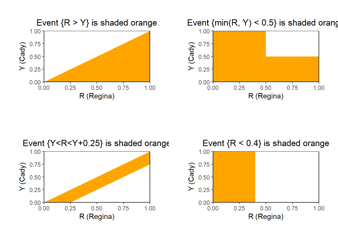
Figure 2.4: Illustration of the events in Exercise 2.15. The square represents the possible values of \((R, Y)\), the random vector representing the arrival times of Regina and Cady.
Outcomes, events, and random variables are some of the main objects of probability. While they are related, these are distinct objects. Mathematically, an outcome is a point, an event is a set, and a random variable is a function. As such, different operations are valid depending on what you’re dealing with. Don’t confuse operations like \(\cap\) that operate on sets (events, “and”) with operations like \(+\) that operate on numbers and functions (random variables, “plus” meaning addition).
Example 2.16 At various points in his homework, Donny Don’t writes the following. Explain to Donny why each of the following symbols is nonsense, both mathematically and intuitively using a simple example (like tomorrow’s weather). Below, \(A\) and \(B\) represent events, \(X\) and \(Y\) represent random variables.
- \(A = 0.5\)
- \(A + B\)
- \(X = A\)
- \(X + A\)
- \(X \cap Y\)
Solution. to Example 2.16
Show/hide solution
We’ll respond to Donny using tomorrow’s weather as an example, with \(A\) representing the event that it rains tomorrow, \(X\) tomorrow’s high temperature (degrees F), \(B=\{X>80\}\) the event that tomorrow’s high temperature is above 80 degrees, and \(Y\) tomorrow’s rainfall (inches).
- \(A\) is a set and 0.5 is a number; it doesn’t make mathematical sense to equate them. It doesn’t make sense to say “it rains tomorrow equals 0.5”.
- \(A\) and \(B\) are sets; it doesn’t make mathematical sense to add them. It doesn’t make sense to say “the sum of (it rains tomorrow) and (tomorrow’s high temperature is above 80 degrees F)”. If we want “(it rains tomorrow) OR (tomorrow’s high temperature is above 80 degrees F)”, then we need \(A\cup B\). Union is an operation on sets; addition is an operation on numbers.
- \(X\) is a random variable (a function) and \(A\) is an event (a set), and it doesn’t make sense to equate these two different mathematical objects. Suppose that \(X\) represents tomorrow’s high temperate (degrees F). It doesn’t make sense to say “tomorrow’s high temperature equals the event that it rains tomorrow”.
- \(X\) is a random variable (a function) and \(A\) is an event (a set), and it doesn’t make sense to add these two different mathematical objects. It doesn’t make sense to say “the sum of (tomorrow’s high temperature) and (the event that it rains tomorrow)”.
- \(X\) and \(Y\) are random variables (functions) and intersection is an operation on sets. \(X \cap Y\) is attempting to say “tomorrow’s high temperature in degrees F and the amount of rainfall in inches tomorrow”. If we’re talking about a random vector containing these two variables, we would write \((X, Y)\) not \(X \cap Y\). If we’re interested in an event involving \(X\) and \(Y\), we’re missing qualifying information to define a valid event. We could write \(X >80, Y < 2\) or \(\{X > 80\} \cap \{Y < 2\}\) to represent “the event that (tomorrow’s high temperature is greater than 80 degrees F) AND (the amount of rainfall tomorrow is less than 2 inches)”.
2.3.1 Summary
- Roughly, a random variable assigns a number measuring some quantity of interest to each outcome of a random phenomenon.
- Mathematically, a random variable is a function whose input is a sample space outcome and whose output is a real number.
- Many events of interest involve random variables.
- A function of a random variable is also a random variable.
- Sums, products, and other transformations of multiple random variables defined on the same sample space are random variables.
- If the sample space outcomes are represented by rows in a spreadsheet, then random variables correspond to columns.