2.5 Introduction to simulation

A probability model of a random phenomenon consists of a sample space of possible outcomes, associated events and random variables, and a probability measure which specifies probabilities of events and determines distributions of random variables. Simulation involves using a probability model to artificially recreate a random phenomenon, many times, usually using a computer. Given a probability model, we can simulate outcomes, occurrences of events, and values of random variables, according to the specifications of the probability measure which reflects the model assumptions.

Recall that probabilities can be interpreted as long run relative frequencies. Therefore the probability of an event can be approximated by simulating, according to the assumptions of the probability model, the random phenomenon a large number of times and computing the relative frequency of repetitions on which the event occurs. Simulation can be used to approximate probabilities of events, distributions of random variables, long run averages, and other characteristics.

In general, a simulation involves the following steps.

Set up. Define a probability space, and related random variables and events. The probability measure encodes all the assumptions of the model, but the probability measure is often only specified indirectly. The set up might be as simple as “flip a fair coin ten times and count the number of heads”. However, even when the set up can be described simply, translating the setup into computer code can be challenging³⁵.
Simulate. Simulate — according to the assumptions reflected in the probability measure — outcomes, occurrences of events, and values of random variables.
Summarize. Summarize simulation output in plots and summary statistics (relative frequencies, averages, standard deviations, correlations, etc) to describe and approximate probabilities, distributions, and related characteristics.
Sensitivity analysis. Investigate how results respond to changes in the assumptions or parameters of the simulation.

You might ask: if we have access to the probability measure, then why do we need simulation to approximate probabilities? Can’t we just compute them? Remember that the probability measure is often only specified indirectly. The probability measure represents the underlying assumptions under which probabilities of events of interest are determined. But in most situations the probability measure does not provide an explicit formula for computing the probability of any particular event. And in many cases, it is impossible to enumerate all possible outcomes. For example, a probabilistic model of a particular Atlantic Hurricane does not provide a mathematical formula for computing the probability that the hurricane makes landfall in the U.S. Nor does the model provide a comprehensive list of the uncountably many possible paths of the hurricane. Rather, the model reflects a set of assumptions under which possible paths can be simulated to approximate probabilities of events of interest.

We will see techniques for computing probabilities, but in many situations explicit computation is difficult. Simulation is a powerful tool for investigating probability models and solving complex problems.

2.5.1 Tactile simulation: Boxes and spinners

While we generally use technology to conduct large scale simulations, it is helpful to first consider how we might conduct a simulation by hand using physical objects like coins, dice, cards, or spinners.

Many random phenomena can be represented in terms of a “box model³⁶”

Imagine a box containing “tickets” with labels. Examples include:
- Fair coin flip. 2 tickets: 1 labeled H and 1 labeled T
- Free throw attempt of a 90% free throw shooter. 10 tickets: 9 labeled “make” and 1 labeled “miss”
- Card shuffling. 52 cards: each card with a pair of labels (face value, suit).
The tickets are shuffled in the box, some number are drawn out — either with replacement or without replacement of the tickets before the next draw³⁷.
In some cases, the order in which the tickets are drawn matters; in other cases the order is irrelevant. For example,
- Dealing a 5 card poker hand: Select 5 cards without replacement, order does not matter
- Random digit dialing: Select 4 cards with replacement from a box with tickets labeled 0 through 9 to represent the last 4 digits of a randomly selected phone number with a particular area code and exchange; order matters, e.g., 805-555-1212 is a different outcome than 805-555-2121.
Then something is done with the tickets, typically to measure random variables of interest. For example, you might flip a coin 10 times (by drawing from the H/T box 10 times with replacement) and count the number of H.

If the draws are made with replacement from a single box, we can think of a single circular “spinner” instead of a box, spun multiple times. For example:

Fair coin flip. Spinner with half of the area corresponding to H and half T
Free throw attempt of a 90% free throw shooter. Spinner with 90% of the area corresponding to “make” and 10% “miss”.

Example 2.26 Let \(X\) be the sum of two rolls of a fair four-sided die, and let \(Y\) be the larger of the two rolls (or the common value if a tie). Set up a box model and explain how you would use it to simulate a single realization of \((X, Y)\). Could you use a spinner instead?

Solution. to Example 2.26

Show/hide solution

Use a box with four tickets, labeled 1, 2, 3, 4. Draw two tickets with replacement. Let \(X\) be the sum of the two numbers drawn and \(Y\) the larger of the two numbers drawn.

It’s also possible to use a spinner with 4 sectors, corresponding to 1, 2, 3, 4, each with 25% of the total area; see Figure 2.12. Spin the spinner twice. Let \(X\) be the sum of the two numbers spun and \(Y\) the larger of the two numbers spun.

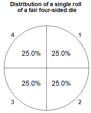
Figure 2.12: Spinner corresponding to a single roll of a fair four-sided die.

The spinner in Figure 2.12 simulates the individual die rolls. We will see later spinners for generating values of \(X\), values of \(Y\), and values of \((X, Y)\) pairs directly.

Note that we are able to simulate outcomes of the rolls and values of \(X\) and \(Y\) without defining the probability space in detail. That is, we do not need to list all the possible outcomes and events and their probabilities. Instead, the probability space is defined implicitly via the specification to “roll a fair four-sided die twice” or “draw two tickets with replacement from a box with four tickets labeled 1, 2, 3, 4” or “spin the spinner in Figure 2.12 twice”. The random variables are defined by what is being measured for each outcome, the sum (\(X\)) and the max (\(Y\)) of the two draws or spins.

In Example 2.26 we described how to simulate a single realization of \((X, Y)\); this is one “repetition” in the simulation. A simulation usually involves many repetitions. When conducting simulations it is important to distinguish between what entails (1) one repetition of the simulation and its output, and (2) the simulation itself and output from many repetitions.

Example 2.27 Consider the matching problem (Example 2.4) with \(n=4\). Label the objects 1, 2, 3, 4, and the spots 1, 2, 3, 4, with spot 1 the correct spot for object 1, etc. Let \(X\) be the number of rocks that are placed in the correct spot, and let \(C\) be the event that at least one rock is placed in the correct spot. Describe how you would use a box model to simulate a single realization of \(Y\) and of \(C\). Could you use a spinner instead?

Solution. to Example 2.27

Show/hide solution

Use a box with 4 tickets, labeled 1, 2, 3, 4. Shuffle the tickets and draw all 4 without replacement and record the tickets drawn in order. Let \(Y\) be the number of tickets that match their spot in order. (For example, if the tickets are drawn in the order 2431 then the realized value of \(X\) is 1 since only ticket 3 matches its spot in the order.)

Since \(C=\{X \ge 1\}\), event \(C\) occurs if \(X\ge 1\) and does not occur if \(X=0\). We could record the realization of event \(C\) as “True” or “False”. We could also record the realization of \(I_C\), the indicator random variable for event \(C\), as 1 if \(C\) occurs and 0 if \(C\) does not occur.

Since the tickets are drawn without replacement, we could not simply spin a single spinner, like the one in Figure 2.12, four times. If we really wanted to use the spinner in Figure 2.12, we couldn’t just spin it four times; we would sometimes have to discard spins and try again. For example, suppose the first spin results in 2; then if the second spin results in 2 would we need to discard it and try again. So we would usually need more than four spins to obtain a valid outcome. If we wanted to guarantee a valid outcome in only four spins, we would need a collection of spinners, and which one we use would depend on the results of previous spins. For example, if the first spin results in 2, then we would need to spin a spinner that only lands on 1, 3, 4; if the second spin results in 3, then we would need to spin and spinner that lands only on 1 and 4.

Example 2.28 Consider a version of the meeting problem (Example 2.3) where Regina and Cady will definitely arrive between noon and 1, but their exact arrival times are uncertain. Rather than dealing with clock time, it is helpful to represent noon as time 0 and measure time as minutes after noon, so that arrival times take values in the continuous interval [0, 60].

Explain how you would construct a spinner and use it to simulate an outcome. Why could we not simulate this situation with a box model?

Solution. to Example 2.28

Show/hide solution

We could construct a spinner like the one in Figure 2.1, but ranging from 0 to 60 instead of 0 to 1; see Figure 2.13. (Or we could just use the spinner in Figure 2.1, but multiply the result of each spin by 60.) Only selected rounded values are displayed on the circular axis, but in the idealized model the spinner is infinitely precise so that any real number between 0 and 60 is a possible outcome. Spin it twice; the first spin represents Regina’s arrival, the second Cady’s.

An outcome consists of a pair of values from the continuous interal [0, 60]. Since this interval is uncountable, it’s not possible to write every real number in the interval [0, 60] on a ticket to place in a box. With a box model, we would have to round arrival times to some desired degree of precision — nearest minute, second, millisecond, etc — and put the rounded values on the tickets. Which is probably fine for practical purposes! But if we really want to create a tactile representation of continuous outcomes, a box model won’t work; we tend to use spinners instead.

Figure 2.13: A continuous [0, 60] spinner. The same spinner is displayed on both sides, with different features highlighted on the left and right. Only selected rounded values are displayed, but in the idealized model the spinner is infinitely precise so that any real number between 0 and 60 is a possible outcome.

Notice that the values on the circular axis in Figure 2.13 are evenly spaced. For example, the intervals [0, 15] and [15, 30], both of length 15, each represent 25% of the spinner area. If we spin the idealized spinner represented by Figure 2.13 10 times, our results might look like the following.

Table 2.15: Results of 10 spins of the Uniform(0, 60) spinner.
Spin	Result
1	32.08970
2	42.46565
3	32.49815
4	17.24412
5	15.21622
6	56.61295
7	50.63507
8	56.59509
9	56.85495
10	48.20989

Notice the number of decimal places. For the Uniform(0, 60) model, any value in the continuous interval between 0 and 60 is a distinct possible value: 10.25000000000… is different from 10.25000000001… is distinct from 10.2500000000000000000001… and so on.

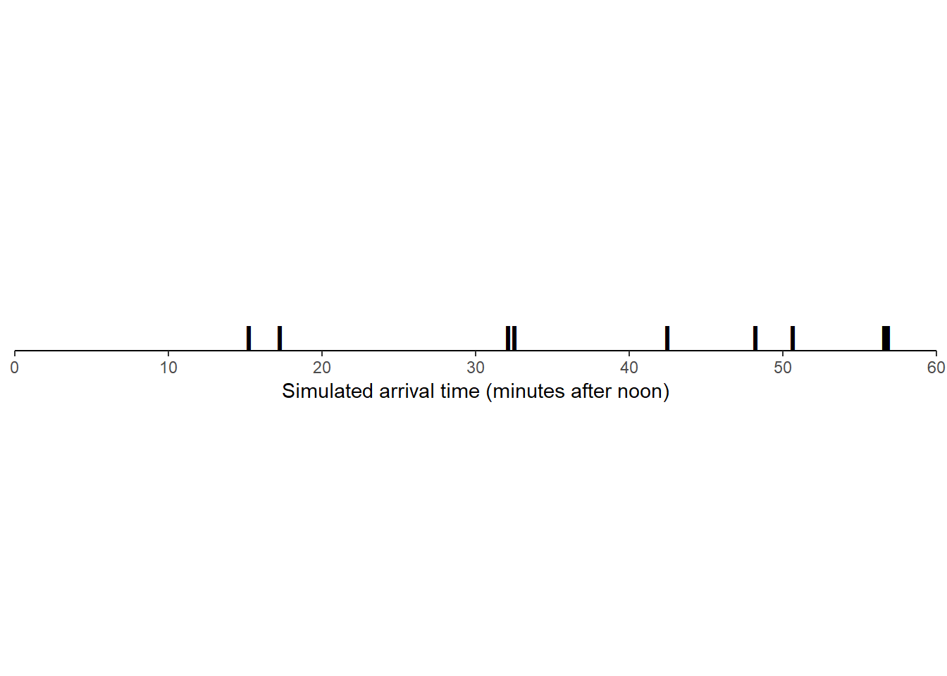
If we plot the 10 simulated values along a number line, they are roughly evenly spaced, though there is some natural variability. (Though it’s hard to discern any patterns with only 10 values.)

To simulate a (Regina, Cady) pair of arrival times, we would spin the Uniform(0, 60) spinner twice. The following displays the results of 10 repetitions, each repetition resulting in a (Regina, Cady) pair.

Table 2.16: Results of 10 pairs of spins of the Uniform(0, 60) spinner.
Repetition	Regina’s time	Cady’s time
1	37.42935	24.21099
2	19.53416	40.85437
3	16.40402	11.04373
4	29.29765	22.17613
5	18.05499	48.57052
6	27.56311	25.33058
7	13.55824	59.47177
8	22.57686	36.87912
9	10.74590	19.37393
10	52.92529	36.60642

Here is a plot of the 10 simulated pairs of arrival times.

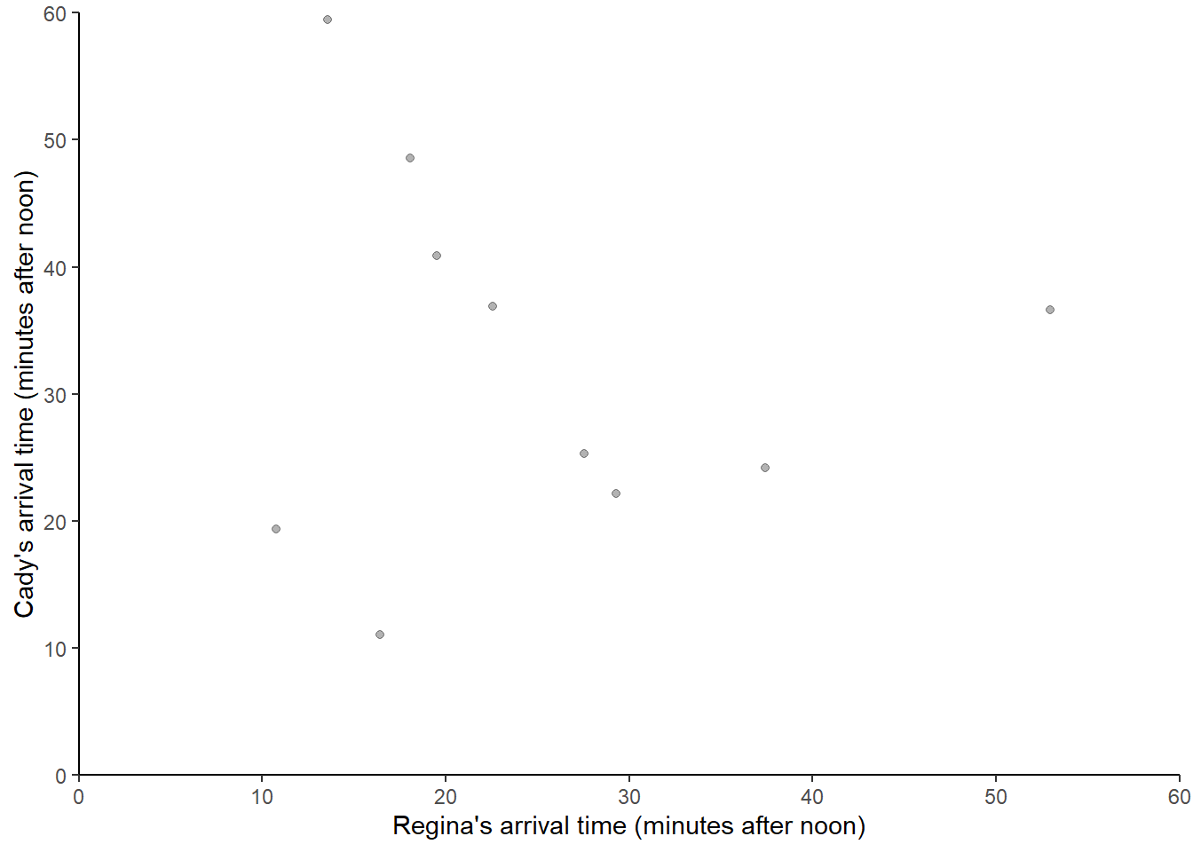
Now suppose we keep repeating the process, resulting in many simulated (Regina, Cady) pairs of arrival times. The following displays 1000 simulated pairs of (Regina, Cady) arrival times, resulting from 1000 pairs of spins of the Uniform(0, 60) spinner.

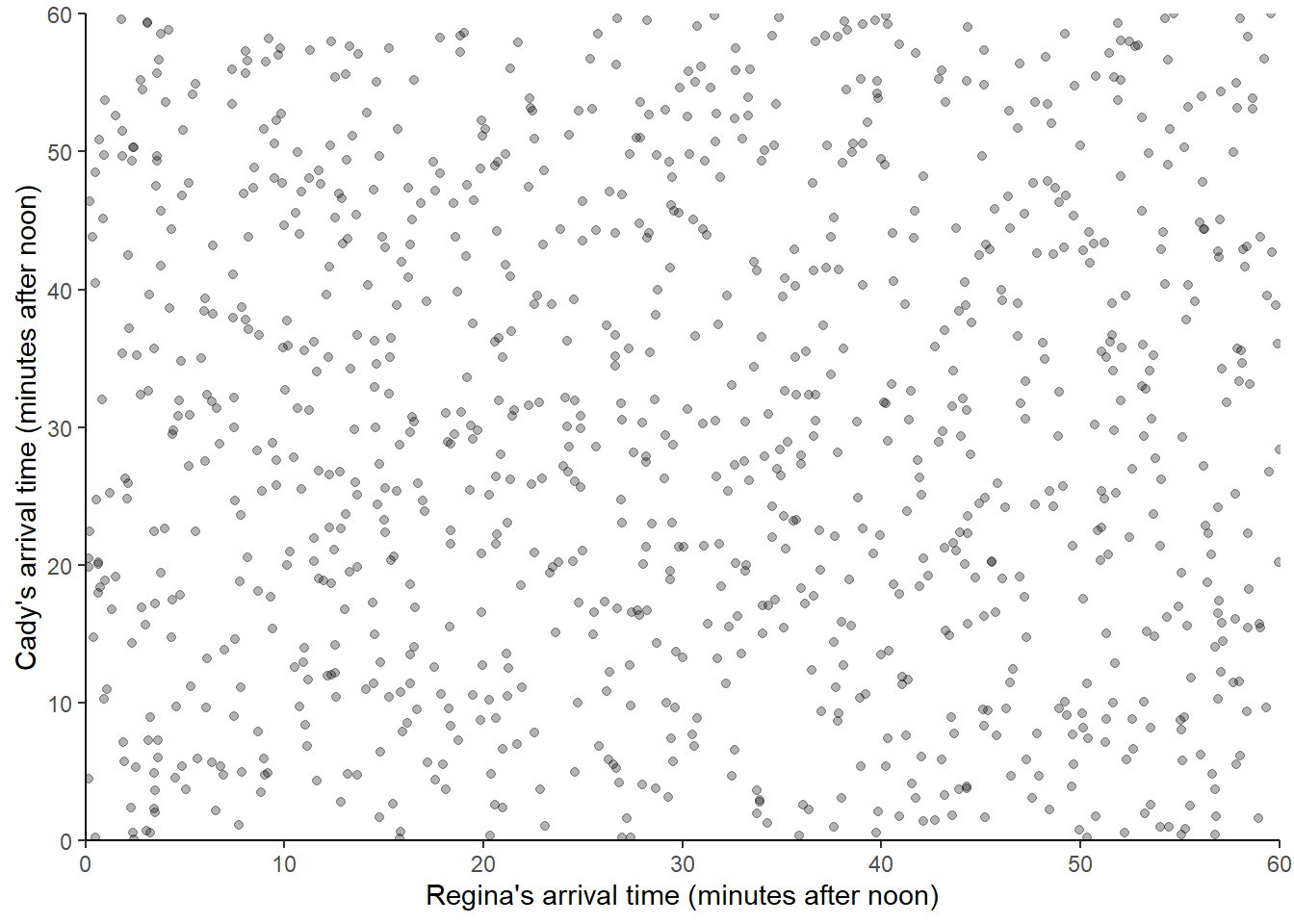
We see that the pairs are fairly evenly distributed throughout the square with sides [0, 60] representing the sample space. If we simulated more values and summarized them in an appropriate plot, we would expect to see something like Figure 2.7.

Now suppose Regina is more likely to arrive around 12:30 than around 12:00 or 1:00. We could construct a spinner that is more likely to land near 30 and less likely to land near 0 or 60. We can do this by “stretching and shrinking” the labels on the circular axis to match our assumptions. Consider the spinner in Figure 2.14. Again, only selected rounded values are displayed in the picture, but the spinner represents an idealized model where the needle is “equally likely” to point to any value in the interval [0, 60]. But pay close attention to the circular axis; the values are not equally spaced. For example, the bottom half of the spinner corresponds to the interval [23.26, 36.74], with length 13.48 minutes, while the upper half of the spinner corresponds to the intervals [0, 23.26] and [36.74, 60], with total length 46.52 minutes. Compared with the Uniform(0, 60) spinner, in the Normal(30, 10) spinner intervals near 30 are “stretched out” to reflect a higher probability of arriving near 12:30, while intervals near 0 and 60 are “shrunk” to reflect a lower probability of arrival near 12:00 or 1:00. For example, the interval [20, 40] represent about 68% of the spinner area, so if we spin this spinner many times, about 68% of the arrival times will be in the interval [20, 40]. (The spinner is divided into 16 wedges of equal area, so each wedge represents 6.25% of the probability. Not all values on the axis are labeled, but you can use the wedges to eyeball probabilities.) That is, according to this model Regina has a 68% chance of arriving within 10 minutes of 12:30, compared to a 33% chance in the Uniform(0, 60) model.

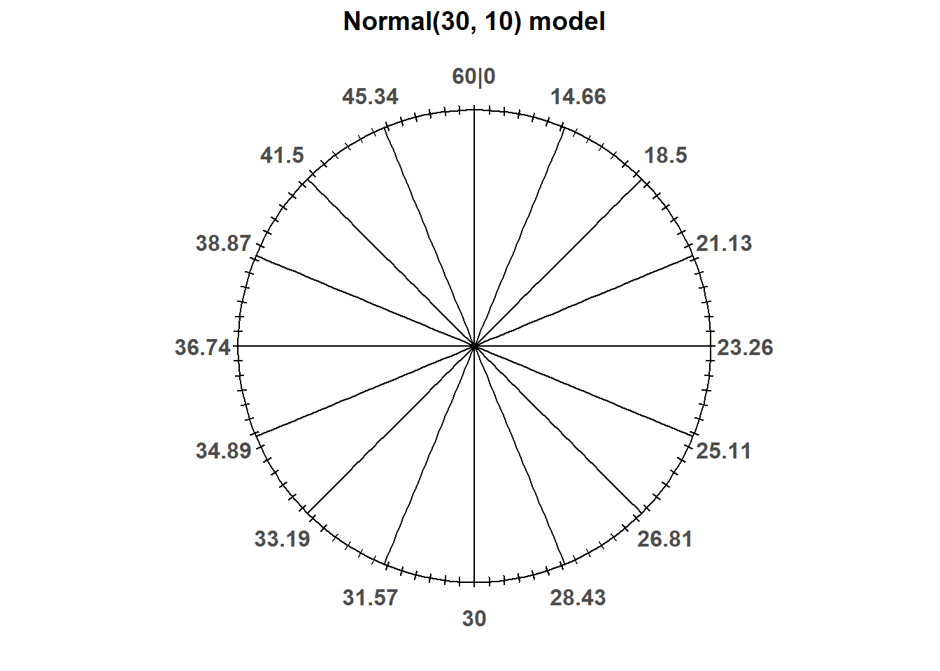
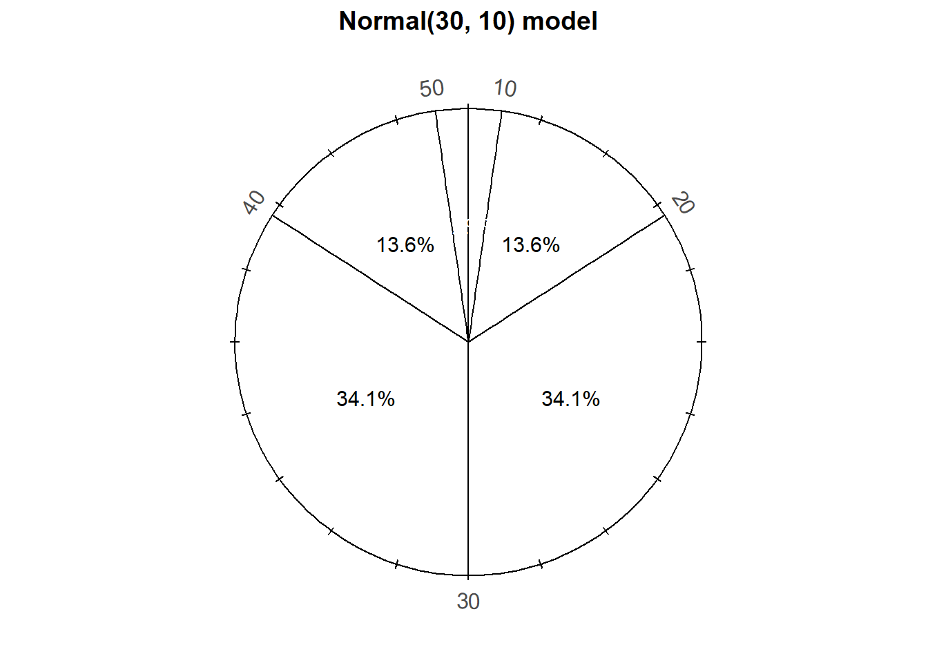
Figure 2.14: A continuous Normal(30, 10) spinner. The same spinner is displayed on both sides, with different features highlighted on the left and right. Only selected rounded values are displayed, but in the idealized model the spinner is infinitely precise so that any real number is a possible outcome. Notice that the values on the axis are not evenly spaced.

The particular pattern represented by the spinner in Figure 2.14 is a Normal(30, 10) distribution; that is, a Normal distribution with mean 30 and standard deviation 10. (Note: technically this allows for some arrival times outside the [0, 60] interval.) We will see Normal distributions in much more detail in the future; in this section we simply introduce them as one way to move beyond Uniform models. For now, just know that a Normal(30, 10) reflects one particular pattern of variability. The following table compares probabilities of selected intervals under the Uniform(0, 60) and Normal(30, 10) models³⁸.

Comparison of probabilities for the Uniform(0, 60) and Normal(30, 10) spinners
Interval	Uniform(0, 60) probability	Normal(30, 10) probability
[0. 10]	16.67%	2.5%
[10, 20]	16.67%	13.6%
[20, 30]	16.67%	34.1%
[30. 40]	16.67%	34.1%
[40, 50]	16.67%	13.6%
[50, 60]	16.67%	2.5%

If we spin the idealized spinner represented by Figure 2.14 10 times, our results might look like the following.

Table 2.17: Results of 10 spins of the Normal(30, 10) spinner.
Spin	Result
1	39.97481
2	17.73089
3	40.54407
4	31.72622
5	19.77891
6	32.86916
7	46.84994
8	22.46540
9	38.35594
10	33.41538

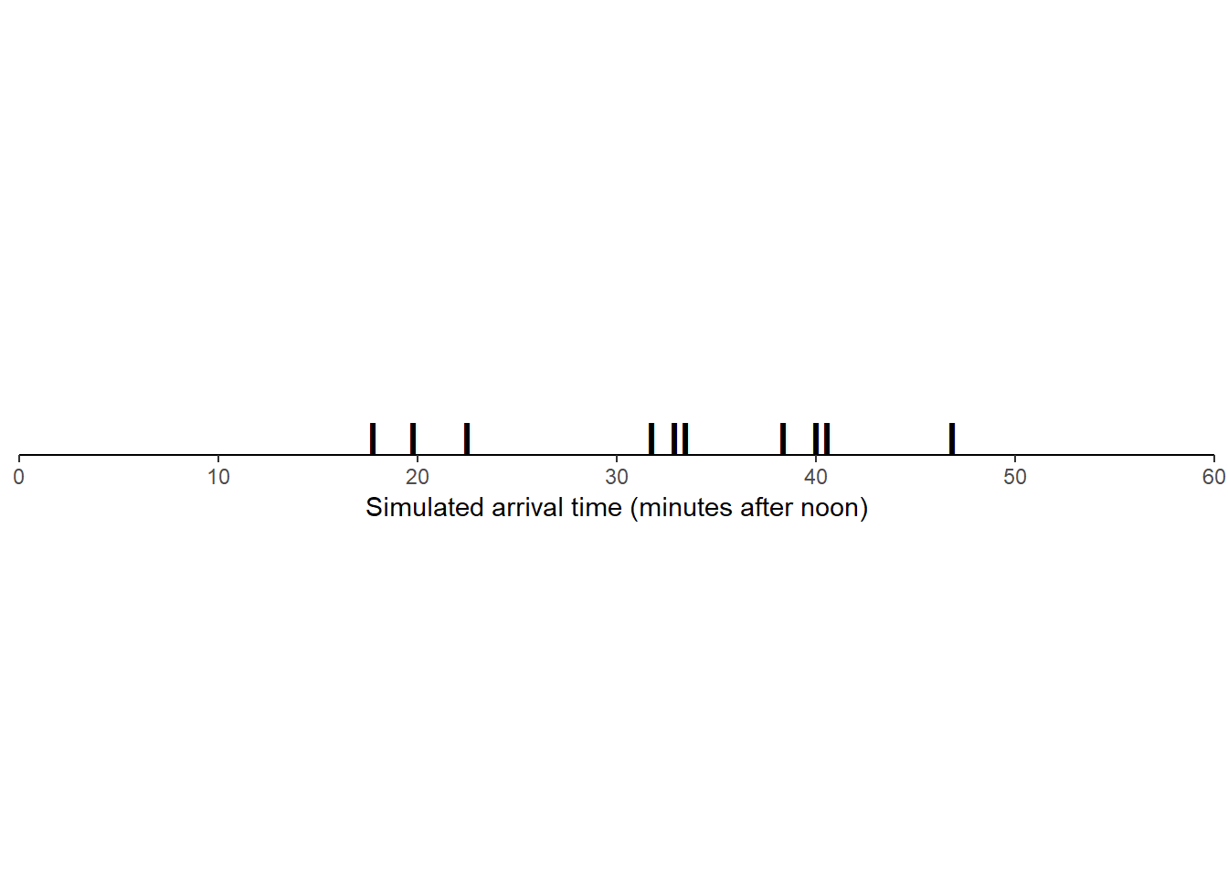
If we plot the 10 simulated values along a number line, we tend to see more values near 30 than near 0 or 60. (Again, it’s hard to discern any patterns with only 10 values.)

Regina’s and Cady’s arrival times are each reasonably modeled by a Normal(30, 10) model, independently of each other. To simulate a (Regina, Cady) pair of arrival times, we would spin the Normal(30, 10) spinner twice. The following displays the results of 10 repetitions, each repetition resulting in a (Regina, Cady) pair.

Table 2.18: Results of 10 pairs of spins of the Normal(30, 10) spinner.
Repetition	Regina’s time	Cady’s time
1	25.91455	37.79797
2	34.59920	34.29835
3	48.52812	35.53131
4	44.46270	43.25082
5	30.97264	42.19464
6	24.55201	40.67761
7	17.82223	30.14482
8	38.74022	41.88868
9	31.80029	43.79792
10	34.39579	40.58755

Here is a plot of the 10 simulated pairs of arrival times.

The following plots 1000 pairs of (Regina, Cady) arrival times, resulting from 1000 pairs of spins of the Normal(30, 10) spinner.

## Warning: Removed 6 rows containing missing values (geom_point).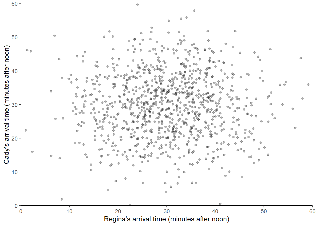

Compared with the simulated pairs from the Uniform(0, 60) spinner, we see many more simulated pairs in the center of the plot (when both arrive near 12:30) than in the corners of the plot (where either arrives near 12:00 or 1:00). If we simulated more values and summarized them in an appropriate plot, we would expect to see something like Figure 2.10.

Recall that Figure 2.11 reflected a model where Regina and Cady each are more likely to arrive around 12:30 than noon or 1:00, but they coordinate their arrivals so they are more likely to arrive around the same time. In such a situation, we could use spinners to simulate pairs of arrival times, but it’s more involved than just spinning a single spinner twice. We revisit using spinners to simulate dependent pairs later.

2.5.2 Computer simulation: Dice rolling

Note: some of the plots and tables in this and the following sections do not appear exactly as they would in Jupyter or Colab notebooks.

We will perform computer simulations using the Python package Symbulate. The syntax of Symbulate mirrors the language of probability in that the primary objects in Symbulate are the same as the primary components of a probability model: probability spaces, random variables, events. Once these components are specified, Symbulate allows users to simulate many times from the probability model and summarize the results.

This section contains a brief introduction to Symbulate; more examples can be found throughout the text or in the Symbulate documentation. Remember to first import Symbulate during a Python session using the command

from symbulate import *

We’ll start with a dice rolling example. Unless indicated otherwise, in this section \(X\) represents the sum of two rolls of a fair four-sided die, and \(Y\) represents the larger of the two rolls (or the common value if a tie). We have already discussed a tactile simulation; now we have to implement that process on a computer.

2.5.2.1 Simulating outcomes

The following Symbulate code defines a probability space³⁹ P for simulating the 16 equally likely ordered pairs of rolls via a box model.


P = BoxModel([1, 2, 3, 4], size = 2, replace = True)

The above code tells Symbulate to draw 2 tickets (size = 2), with replacement⁴⁰, from a box with tickets labeled 1, 2, 3, and 4 (entered as the Python list [1, 2, 3, 4]). Each simulated outcome consists of an ordered⁴¹ pair of rolls .

The sim(r) command simulates `r`` realizations of probability space outcomes (or events or random variables). Here is the result of one repetition.


P.sim(1)

Index	Result
0	(2, 4)

And here are the results of 10 repetitions. (We will typically run thousands of repetitions, or more, but in this section we just run a few repetitions for illustration.)


P.sim(10)

Index	Result
0	(2, 1)
1	(3, 3)
2	(2, 4)
3	(4, 3)
4	(2, 2)
5	(2, 2)
6	(3, 3)
7	(2, 1)
8	(1, 1)
...	...
9	(1, 2)

One important note is that every time .sim() is called, a new simulation is run. When running a simulation, the “simulate” step should be performed with a single call to sim so that all analysis of results corresponds to the same simulated values.

2.5.2.2 Simulating random variables

A Symbulate RV is specified by the probability space on which it is defined and the mapping function which defines it. Recall that \(X\) is the sum of the two dice rolls and \(Y\) is the larger (max).

X = RV(P, sum)
Y = RV(P, max)

The above code simply defines the random variables. Again, we can simulate values with .sim(). Since every call to sim runs a new simulation, we typically store the simulation results as an object. The following commands simulate 100 values of the random variable X and store the results as x. For consistency with standard probability notation⁴², the random variable itself is denoted with an uppercase letter Y, while the realized values of it are denoted with a lowercase letter y.

x = X.sim(100)

x # this just displays x

Index	Result
0	2
1	6
2	5
3	5
4	4
5	7
6	8
7	6
8	5
...	...
99	6

2.5.2.3 Simulating multiple random variables

if we call X.sim(10000) and Y.sim(10000) we get two separate simulations of 10000 pairs of rolls, one which returns the sum of the rolls for each repetition, and the other the max. If we want to study relationships between \(X\) and \(Y\) we need to compute both \(X\) and \(Y\) for each pair of rolls in the same simulation.

We can simulate \((X, Y)\) pairs using⁴³ &. We store the simulation output as x_and_y to emphasize that x_and_y contains pairs of values.

x_and_y = (X & Y).sim(10)

x_and_y # this just displays x_and_y

Index	Result
0	(5, 3)
1	(5, 3)
2	(6, 3)
3	(4, 2)
4	(5, 4)
5	(4, 2)
6	(2, 1)
7	(3, 2)
8	(4, 3)
...	...
9	(5, 4)

2.5.2.4 Simulating outcomes and random variables

When calling X.sim(10) or (X & Y).sim(10) the outcomes of the rolls are generated in the background but not saved. We can create a RV which returns the outcomes of the probability space⁴⁴. The default mapping function for RV is the identity function, \(g(u) = u\), so simulating values of U = RV(P) below returns the outcomes of the BoxModel P representing the outcome of the two rolls.

U = RV(P)

U.sim(10)

Index	Result
0	(1, 3)
1	(2, 1)
2	(4, 1)
3	(3, 2)
4	(1, 2)
5	(4, 4)
6	(1, 4)
7	(3, 1)
8	(4, 2)
...	...
9	(2, 1)

Now we can simulate and display the outcomes along with the values of \(X\) and \(Y\) using &.

(U & X & Y).sim(10)

Index	Result
0	((3, 3), 6, 3)
1	((4, 1), 5, 4)
2	((1, 1), 2, 1)
3	((2, 1), 3, 2)
4	((4, 2), 6, 4)
5	((4, 1), 5, 4)
6	((4, 2), 6, 4)
7	((2, 4), 6, 4)
8	((4, 3), 7, 4)
...	...
9	((2, 4), 6, 4)

Because the probability space P returns pairs of values, U = RV(P) above defines a random vector. The individual components⁴⁵ of U can be “unpacked” as U1, U2 in the following. Here U1 is an RV representing the result of the first roll and U2 the second.

U1, U2 = RV(P)
(U1 & U2 & X & Y).sim(10)

Index	Result
0	(4, 4, 8, 4)
1	(3, 3, 6, 3)
2	(2, 2, 4, 2)
3	(3, 3, 6, 3)
4	(4, 1, 5, 4)
5	(2, 3, 5, 3)
6	(4, 3, 7, 4)
7	(4, 4, 8, 4)
8	(3, 1, 4, 3)
...	...
9	(4, 1, 5, 4)

2.5.2.5 Simulating events

Events involving random variables can also be defined and simulated. For programming reasons, events are enclosed in parentheses () rather than braces \(\{\}\). For example, we can define the event that the larger of the two rolls is less than 3, \(A=\{Y<3\}\), as

A = (Y < 3) # an event

We can use sim to simulate events. A realization of an event is True if the event occurs for the simulated outcome, or False if not.

A.sim(10)

Index	Result
0	False
1	False
2	True
3	False
4	True
5	False
6	True
7	False
8	False
...	...
9	True

For logical equality use a double equal sign ==. For example, (Y == 3) represents the event \(\{Y=3\}\).

(Y == 3).sim(10)

Index	Result
0	False
1	False
2	True
3	False
4	False
5	True
6	False
7	False
8	False
...	...
9	False

2.5.2.6 Simulating transformations of random variables

Transformations of random variables are random variables. If X is a Symbulate RV and g is a function, then g(X) is also a Symbulate RV.

For example, we can simulate values of \(X^2\).

(X ** 2).sim(10)

Index	Result
0	16
1	25
2	36
3	36
4	16
5	36
6	64
7	4
8	16
...	...
9	16

For many common functions, the syntax g(X) is sufficient. Here exp(u) is the exponential function \(g(u) = e^u\).

(X & exp(X)).sim(10)

Index	Result
0	(4, 54.598150033144236)
1	(6, 403.4287934927351)
2	(3, 20.085536923187668)
3	(6, 403.4287934927351)
4	(5, 148.4131591025766)
5	(3, 20.085536923187668)
6	(5, 148.4131591025766)
7	(3, 20.085536923187668)
8	(8, 2980.9579870417283)
...	...
9	(5, 148.4131591025766)

For user defined functions, the syntax is X.apply(g).

def g(u):
  return (u - 5) ** 2
  
Z = X.apply(g)

(X & Z).sim(10)

Index	Result
0	(5, 0)
1	(8, 9)
2	(5, 0)
3	(4, 1)
4	(6, 1)
5	(2, 9)
6	(3, 4)
7	(3, 4)
8	(2, 9)
...	...
9	(4, 1)

(We could have actually defined Z = (X - 5) ** 2 here. We’ll see examples where the apply syntax is necessary later.)

We can also apply transformations of multiple RVs defined on the same probability space. (We will look more closely at how Symbulate treats this “same probability space” issue later.)

For example, we can simulate values of \(XY\), the product of \(X\) and \(Y\).

(X * Y).sim(10)

Index	Result
0	2
1	15
2	15
3	6
4	18
5	6
6	12
7	24
8	20
...	...
9	12

Recall that we defined \(X\) via X = RV(P, sum). Defining random variables \(U_1, U_2\) to represent the individual rolls, we can define \(X=U_1 + U_2\). Recall that we previously defined⁴⁶ U1, U2 = RV(P).

X = U1 + U2

X.sim(10)

Index	Result
0	7
1	4
2	7
3	3
4	7
5	3
6	6
7	5
8	6
...	...
9	4

Unfortunately max(U1, U2) does not work, but we can use the apply syntax. Since we want to apply max to \((U_1, U_2)\) pairs, we must⁴⁷ first join them together with &.

Y  = (U1 & U2).apply(max)

Y.sim(10)

Index	Result
0	1
1	3
2	4
3	2
4	4
5	2
6	4
7	3
8	4
...	...
9	2

2.5.2.7 Two “worlds” in Symbulate

Suppose we want to simulate realizations of the event \(A= \{Y < 3\}\). We saw previously that we can define the event (Y < 3) in Symbulate and simulate True/False realizations of it.

A = (Y < 3)

A.sim(10)

Index	Result
0	False
1	False
2	True
3	False
4	False
5	False
6	False
7	False
8	False
...	...
9	True

Since event \(A\) is defined in terms of \(Y\), we can also first simulate values of Y, store the results as y, and then determine whether event \(A\) occurs for the simulated y values using⁴⁸ (y < 3). (The results won’t match the above because we are making a new call to sim.)

y = Y.sim(10)

(y < 3)

Index	Result
0	True
1	True
2	False
3	False
4	False
5	False
6	False
7	True
8	False
...	...
9	False

These two methods illustrate the two “worlds” of Symbulate, which we call “random variable world” and “simulation world”. Operations like transformations can be performed in either world. Think of random variable world as the “before” world and simulation world as the “after” world, by which we mean before/after the sim step.

Most of the transformations we have seen so far happened in random variable world. For example, we have seen how to define the sum of two dice in random variable world in a few ways, e.g., via

P = BoxModel([1, 2, 3, 4], size = 2)
U = RV(P)

X = U.apply(sum)

The sum transformation is applied to define a new random variable X, before the sim step. We could then call, e.g., (U & X).sim(10000).

We could also compute simulated values of the sum in simulation world as follows.

P = BoxModel([1, 2, 3, 4], size = 2)
U = RV(P)

u = U.sim(10000)

x = u.apply(sum)

The above code will simulate all the pairs of rolls first, store them as u (which we can think of as a table), and then apply the sum to the simulated values (which adds a column to the table). That is, the sum transformation happens after the sim step.

While either world is “correct”, we generally take the random variable world approach. We do this mostly for consistency, but also to emphasize some of the probability concepts we’ll encounter. For example, the fact that a sum of random variables (defined on the same probability space) is also a random variable is a little more apparent in random variable world. However, it is sometimes more convenient to code in simulation world; for example, if complicated transformations are required.

When working in random variable world, it only makes sense to transform or simulate random variables defined on the same probability space. For example, the following code would return an error.

X = RV(BoxModel([1, 2, 3, 4], size = 2), sum)
Y = RV(BoxModel([1, 2, 3, 4], size = 2), max)

(X & Y).sim(10) # returns an error: "random variables must be defined on the same probability space"

The problem is that there is one box model used to determine values of X and a separate box model for Y; we can’t simulate (X, Y) pairs of values if we’re using different boxes.

Likewise, in simulation world, it only makes sense to apply transformations to values generated in the same simulation, with a single sim step. For example, the following code would return an error.

P = BoxModel([1, 2, 3, 4], size = 2)
U1, U2 = RV(P)

u1 = U1.sim(10000)
u2 = U2.sim(10000)

x = u1 + u2 # returns an error: "objects must come from the same simulation"

We’ll discuss reasons for errors like these in more detail as we go. In short, the “simulation” step should be implemented in a single call to sim.

2.5.2.8 Other probability spaces

So far we have assumed a fair four-sided die. Now consider the weighted die in Example 2.21: a single roll results in 1 with probability 1/10, 2 with probability 2/10, 3 with probability 3/10, and 4 with probability 4/10. BoxModel assumes equally likely tickets by default, but we can specify non-equally likely tickets using the probs option. The probability space WelghtedRoll in the following code corresponds to a single roll of the weighted die; the default size option is 1.


WeightedRoll = BoxModel([1, 2, 3, 4], probs = [0.1, 0.2, 0.3, 0.4])
WeightedRoll.sim(10)

Index	Result
0	2
1	3
2	4
3	1
4	4
5	3
6	4
7	3
8	4
...	...
9	3

We could add size = 2 to the BoxModel to create a probability space corresponding to two rolls of the weighted die. Alternatively, We can also think of BoxModel([1, 2, 3, 4], probs = [0.1, 0.2, 0.3, 0.4]) as defining the middle spinner in Figure 2.6 that we want to spin two times, which we can do with ** 2.

Q = BoxModel([1, 2, 3, 4], probs = [0.1, 0.2, 0.3, 0.4]) ** 2
Q.sim(10)

Index	Result
0	(4, 3)
1	(1, 3)
2	(4, 2)
3	(3, 2)
4	(4, 4)
5	(1, 4)
6	(2, 4)
7	(3, 3)
8	(4, 2)
...	...
9	(3, 2)

For now you can interpret BoxModel([1, 2, 3, 4], probs = [0.1, 0.2, 0.3, 0.4]) as defining the middle spinner in Figure 2.6 and ** 2 as “spin the spinner two times”. In Python, ** represents exponentiation; e.g., 2 ** 5 = 32. So BoxModel([1, 2, 3, 4]) ** 2 is equivalent to BoxModel([1, 2, 3, 4]) * BoxModel([1, 2, 3, 4]). Future sections will reveal why the product * notation is natural for independent spins of spinners.

We could use the product notation to define a probability space corresponding to a pair of rolls: one from a fair die and one from a weighted-die.

MixedRolls = BoxModel([1, 2, 3, 4]) * BoxModel([1, 2, 3, 4], probs = [0.1, 0.2, 0.3, 0.4])
MixedRolls.sim(10)

Index	Result
0	(4, 4)
1	(3, 4)
2	(2, 1)
3	(4, 3)
4	(1, 3)
5	(3, 2)
6	(1, 4)
7	(4, 2)
8	(3, 4)
...	...
9	(3, 3)

Now consider the weighted die from Example 2.22, represented by the spinner on the right in Figure 2.6. We could use the probs option, but we can also imagine a box model with 15 tickets — four tickets labeled 1, six tickets labeled 2, three tickets labeled 3, and two tickets labeled 4 — from which a single ticket is drawn. A BoxModel can be specified in this way using the following {label: number of tickets with the label} formulation⁴⁹. This formulation is especially useful when multiple tickets are drawn from the box without replacement.


Q = BoxModel({1: 4, 2: 6, 3: 3, 4: 2})
Q.sim(10)

Index	Result
0	4
1	3
2	2
3	2
4	3
5	3
6	4
7	2
8	2
...	...
9	1

While many scenarios can be represented by box models, there are also many Symbulate probability spaces other than BoxModel. When tickets are equally likely and sampled with replacement, a Discrete Uniform model can also be used. Think of a DiscreteUniform(a, b) probability space corresponding to a spinner with sectors of equal area labeled with integer values from a to b (inclusive). For example, the spinner in Figure 2.12 corresponds to DiscreteUniform(1, 4). This gives us another way to represent the probability space corresponding to two rolls of a fair-four sided die.

P = DiscreteUniform(1, 4) ** 2
P.sim(10)

Index	Result
0	(4, 3)
1	(1, 2)
2	(3, 4)
3	(3, 3)
4	(4, 4)
5	(3, 3)
6	(3, 4)
7	(4, 4)
8	(3, 2)
...	...
9	(2, 1)

Note that BoxModel is the only probability space with the size argument. For other probability spaces, the product * or exponentiation ** notation must be used to simulate multiple spins.

2.5.3 Computer simulation: Meeting problem

Now we’ll consider a continuous example.

Regina and Cady plan to meet for lunch between noon and 1 but they are not sure of their arrival times. Recall the sample space from Example 2.6. Let \(R\) be the random variable representing Regina’s arrival time (minutes after noon), and \(Y\) for Cady. Also let \(T=\min(R, Y)\) be the time (minutes after noon) at which the first person arrives, and \(W=|R-Y|\) be the time (minutes) the first person to arrive waits for the second person arrives. We’ll simulate these random variables under different assumptions, like those in Section 2.4.2.

Suppose that Regina and Cady arrive uniformly at random between time 0 and 60, independently of each other. Uniform probability measures are the continuous analog of equally likely outcomes. The standard uniform model is the Uniform(0, 1) distribution corresponding to the spinner in Figure 2.1 which returns values between⁵⁰ 0 and 1. Recall that the values in the picture are rounded to two decimal places, but the spinner represents an idealized model where the spinner is infinitely precise so that any real number between 0 and 1 is a possible value. We assume that the (infinitely fine) needle is “equally likely” to land on any value between 0 and 1. A Uniform(\(a\), \(b\)) model⁵¹ is defined similarly for the interval \([a, b]\).

The following code defines a Uniform(0, 60) spinner, like in Figure 2.13, which we spin twice to get the (Regina, Cady) pair of outcomes.

P = Uniform(0, 60) ** 2
P.sim(10)

Index	Result
0	(24.122486301118848, 22.525883426481073)
1	(27.992995952420145, 10.38288584371934)
2	(16.38753054546171, 19.172141952114863)
3	(15.717902206472598, 35.993755837034996)
4	(14.65288693447074, 1.2564850223207147)
5	(44.230028456871466, 49.51467006877388)
6	(19.30641141164314, 4.876806836056449)
7	(52.97127987123101, 19.3746989948418)
8	(25.77107659288081, 36.23555949064066)
...	...
9	(24.50415237442866, 3.8144342795167607)

A probability space outcome is a (Regina, Cady) pair of arrival times. We can define the random variables \(R\) and \(Y\), representing the individual arrive times, by “unpacking” the outcomes.

R, Y = RV(P)
(R & Y).sim(10)

Index	Result
0	(30.817289675448798, 44.03438367586538)
1	(54.289453707807, 55.71933135174607)
2	(21.48977810405967, 0.7311994705864544)
3	(11.309704887993174, 43.69266867158575)
4	(59.58292338841791, 33.670883574874935)
5	(37.04442986126941, 10.585401173866714)
6	(7.38869540547914, 18.956799834251008)
7	(15.055628292291974, 20.088638590613122)
8	(46.806365589058224, 43.80192202019799)
...	...
9	(51.390548386891346, 29.67143868208263)

We can define \(W = |R-Y|\) using the abs function. In order to define \(T = \min(R, Y)\) we need to use the apply syntax with R & Y.

W = abs(R - Y)

T = (R & Y).apply(min)

(R & Y & T & W).sim(10)

Index	Result
0	(57.5292309562332, 27.961083674388444, 27.961083674388444, 29.568147281844755)
1	(2.3753172318480154, 26.111050757694542, 2.3753172318480154, 23.735733525846527)
2	(53.20294292911738, 4.843142283063604, 4.843142283063604, 48.35980064605377)
3	(22.778994424201453, 13.396838884521244, 13.396838884521244, 9.382155539680209)
4	(13.152017766690136, 32.24839430020074, 13.152017766690136, 19.0963765335106)
5	(22.966887458802695, 3.5409562130774885, 3.5409562130774885, 19.425931245725206)
6	(8.036407139708954, 10.797964511604174, 8.036407139708954, 2.76155737189522)
7	(53.421578529254354, 56.529251082196616, 53.421578529254354, 3.1076725529422617)
8	(56.31007561341298, 6.418464562258308, 6.418464562258308, 49.89161105115467)
...	...
9	(38.273253446973506, 47.15677516494947, 38.273253446973506, 8.883521717975967)

Before investigating other assumptions, let’s look at plots of some simulated values. We can simulate values of \(R\) and plot them along a number line. (This plot is called a “rug” plot; we’ll see some more useful plots soon.)

R.sim(100).plot('rug')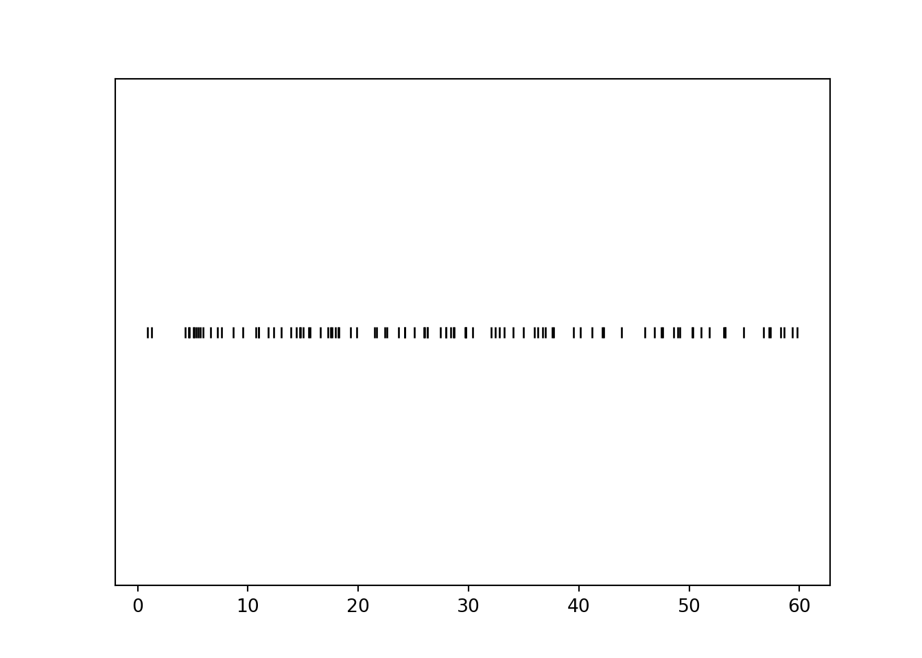

The simulated values are roughly evenly spaced between 0 and 60, though there is some natural variability.

We can simulate and plot many \((R, Y)\) pairs of arrival times.

(R & Y).sim(1000).plot()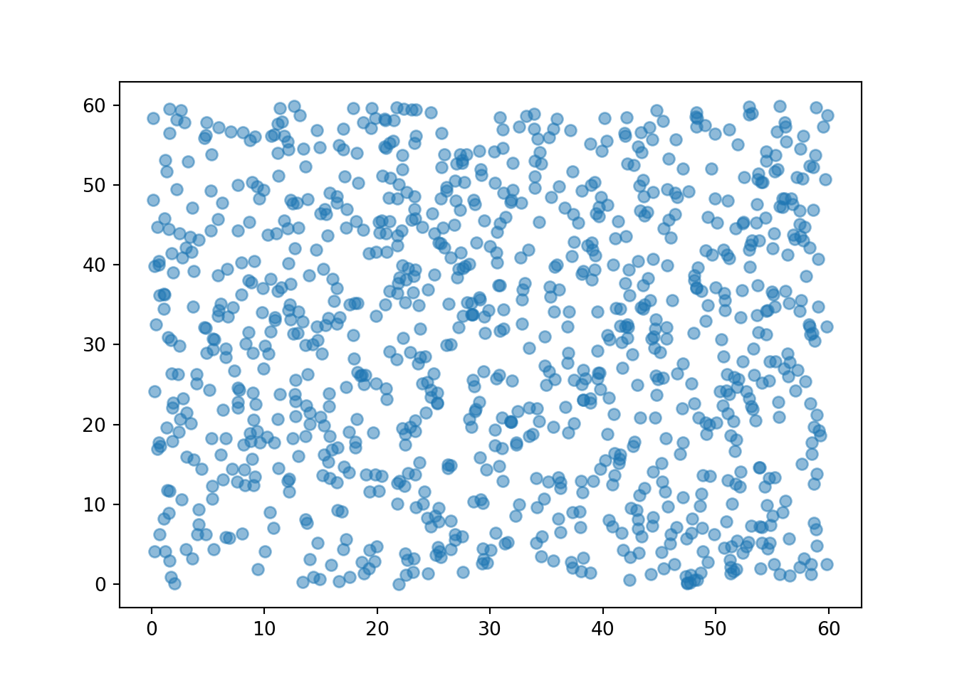

We see that the pairs are fairly evenly distributed throughout the square with sides [0, 60] (which represents the sample space). If we simulated more values and summarized them in an appropriate plot, we would expect to see something like Figure 2.7.

Now suppose Regina is more likely to arrive around 12:30 than around 12:00 or 1:00. One way to model this assumption is with a Normal(30, 10) model, represented by the spinner in like in Figure 2.14.

Normal(mean = 30, sd = 10).sim(10)

Index	Result
0	20.389947048329148
1	41.85233146084762
2	45.89197658304887
3	41.70226557416164
4	9.882217960417194
5	27.003184991465933
6	39.11817497586817
7	40.89324443288544
8	23.18115607301944
...	...
9	30.12909154607931

Now we define a probability space corresponding to (Regina, Cady) pairs of arrival times, by assuming that their arrival times individually follow a Normal(30, 10) model, independently of the other. That is, we spin the Normal(30, 10) spinner twice to simulate a pair of arrival times.

P = Normal(mean = 30, sd = 10) ** 2
P.sim(10)

Index	Result
0	(29.72213530899267, 32.363872689333775)
1	(30.134804146906216, 32.701854538706385)
2	(30.4779948645945, 21.794346375219185)
3	(36.46576339224676, 31.93889836323547)
4	(28.54688089158301, 22.810638841497223)
5	(24.65184958436905, 7.856871748330086)
6	(22.88930774881998, 36.24886970316555)
7	(42.94460179968323, 31.121351193010177)
8	(28.34597843740897, 38.59577709831731)
...	...
9	(13.316875208664879, 28.697681204402084)

We can unpack the individual \(R\), \(Y\) random variables as before.

R, Y = RV(P)

Again, we can simulate values and plot them. Compared to the rug plot based on the Uniform model, the rug plot based on the Normal model shows that more simulated \(R\) values tend to be close to 30 than near 0 or 60.

R.sim(100).plot('rug')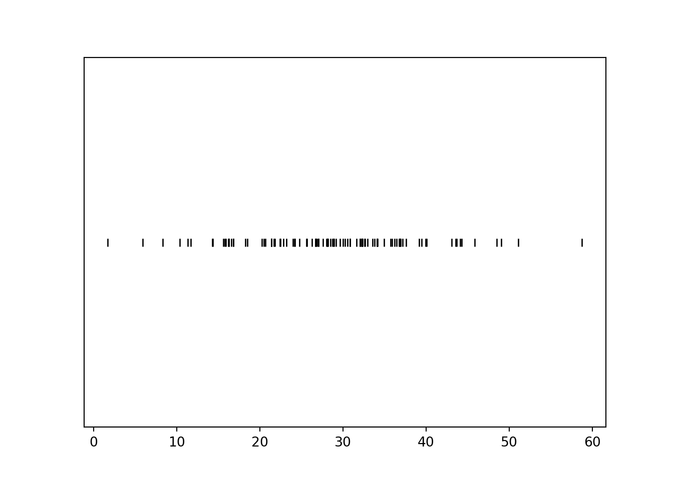

We can simulate and plot \((R, Y)\) pairs.

(R & Y).sim(1000).plot()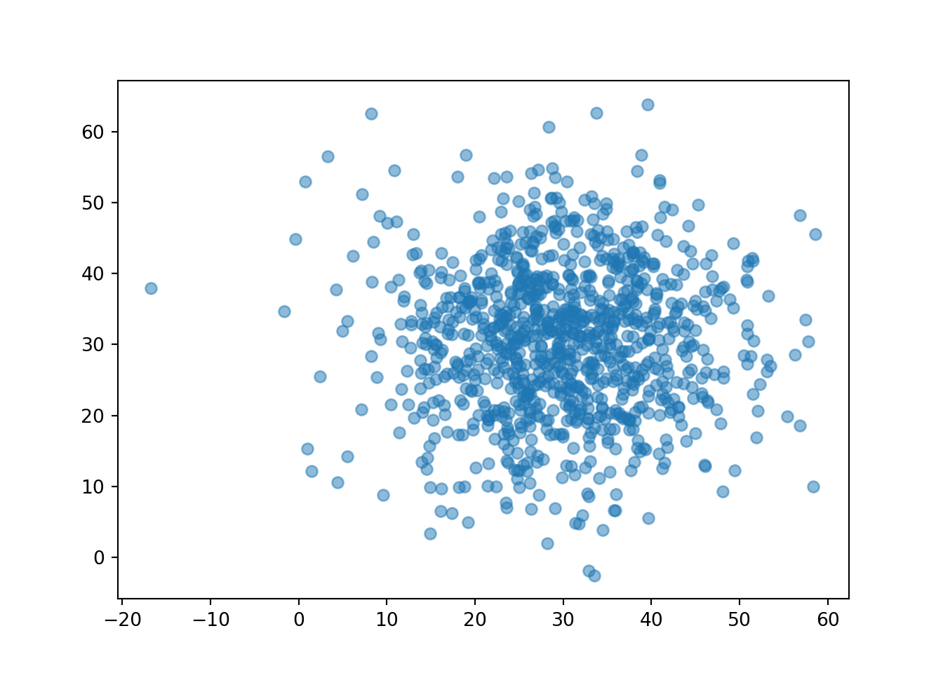

We see that more pairs are located near (30, 30), similar to Figure 2.10. (We also might see some values outside of [0, 60].)

Now suppose we want to also assume that Regina and Cady tend to arrive around the same time. One way to model pairs of values that have correlation is with a BivariateNormal distribution, like in the following.

P = BivariateNormal(mean1 = 30, sd1 = 10, mean2 = 30, sd2 = 10, corr = 0.7)
P.sim(10)

Index	Result
0	(37.69222925100529, 38.5318683094932)
1	(37.35093555589915, 27.71010243556556)
2	(43.08821650127654, 39.16136251038877)
3	(38.474086267827495, 36.119182736039846)
4	(29.77961713177933, 31.38321033734426)
5	(36.12519437804053, 27.812260300105454)
6	(34.92122456541884, 44.87867211635446)
7	(24.03226063273652, 15.726172790437213)
8	(21.819789023091275, 32.89752101122859)
...	...
9	(30.268905002495817, 31.78601791883798)

Note that the BivariateNormal probability space returns pairs directly. We can unpack the pairs, and plot some simulated values.

R, Y = RV(P)

(R & Y).sim(1000).plot()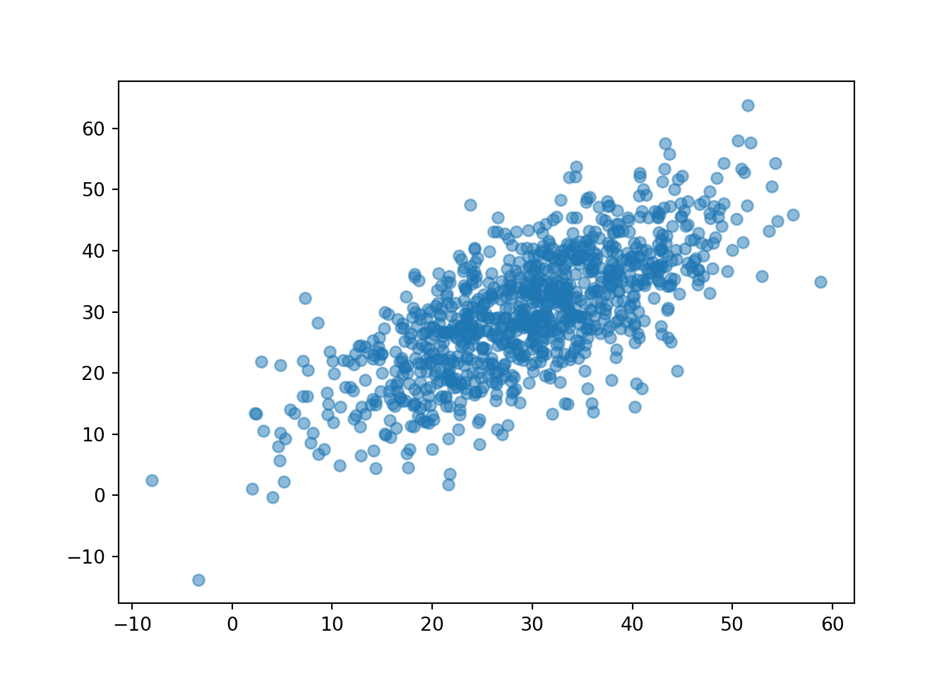

Now we see that the points tend to follow the \(R = Y\) line, so that Regina and Cady tend to arrive near the same time, similar to Figure 2.11.

This section has provided some basic examples of how to define probability spaces and random variables in Symbulate. We will study specific probability models like Normal and BivariateNormal in much more detail as we go.

References

Freedman, David, Robert Pisani, and Roger Purves. 2007. Statistics. 4th ed. W.W. Norton; Company.

In most situations we’ll encounter in this book, the “simulate” and “summarize” steps are usually straightforward. In many other cases, these steps can be challenging. Complex set ups often require sophisticated methods, such MCMC (Markov Chain Monte Carlo) algorithms, to efficiently simulate realizations. Effectively summarizing high dimensional simulation output often requires the use of multivariate statistics and visualizations.↩︎
Our use of “box models” is inspired by (Freedman, Pisani, and Purves 2007).↩︎
“With replacement” always implies replacement at a uniformly random point in the box. Think of “with replacement” as “with replacement and reshuffling” before the next draw.↩︎
Careful: the parameters in the Uniform model are different from those in the Normal model. In the Uniform(0, 60) model, 0 is the minimum possible value; in the Normal(30, 10) model, 30 is the average value. In the Uniform(0, 60) model, 60 is the maximum possible value; in the Normal(30, 10) model, 10 is the standard deviation.↩︎
We primarily view a Symbulate probability space as a description of the probability model rather than an explicit specification of the sample space \(\Omega\). For example, we define a BoxModel instead of creating a set with all possible outcomes. We tend to represent a probability space with P, even though this is a slight abuse of notation (since \(\textrm{P}\) typically refers to a probability measure).↩︎
The default argument for replace is True, so we could have just written BoxModel([1, 2, 3, 4], size = 2).↩︎
There is an additional argument order_matters which defaults to True, but we could set it to False for unordered pairs.↩︎
We generally use names in our code that mirror and reinforce standard probability notation, e.g., uppercase letters near the end of the alphabet for random variables, with corresponding lowercase letters for their realized values. Of course, these naming conventions are not necessary and you are welcome to use more descriptive names in your code. For example, we could have named the probability space DiceRolls and the random variables DiceSum and DiceMax rather than P, X, Y.↩︎
Technically & joins two RVs together to form a random vector. While we often interpret Symbulate RV as random variable, it really functions as random vector.↩︎
You might try (P & X).sim(10). But P is a probability space object, and X is an RV object, and & can only be used to join like objects together. Much like in probability theory in general, in Symbulate the probability space plays a background role, and it is usually random variables we are interested in.↩︎
The components can also be accessed using brackets. U1, U2 = RV(P) is shorthand for
U = RV(P); U1 = U[0]; U2 = U[1]. Python uses zero-based indexing, so 0 refers to the first component, 1 to the second, and so on.↩︎
We can also define U = RV(P) and then X = U.apply(sum).↩︎
We can also define U = RV(P) and then X = U.apply(max).↩︎
Python automatically treats True as 1 and False as 0, so the code (y < 3) effectively returns both True/False realizations of event itself and 1/0 realizations of the corresponding indicator random variable.↩︎
Braces {} are used here because this defines a Python dictionary. But don’t confuse this code with set notation.↩︎
Why is the interval \([0, 1]\) the standard instead of some other range of values? Because probabilities take values in \([0, 1]\). We will see why this is useful in more detail later.↩︎
Careful: don’t confuse Uniform(a, b) with DiscreteUniform(a, b). Uniform(a, b) corresponds to the continuous interval \([a, b]\).↩︎