7.2 Normal distributions
Normal distributions are probably the most important distributions in probability and statistics. We have already seen Normal distributions in many previous examples. In this section we’ll explore properties of Normal distributions in a little more depth.
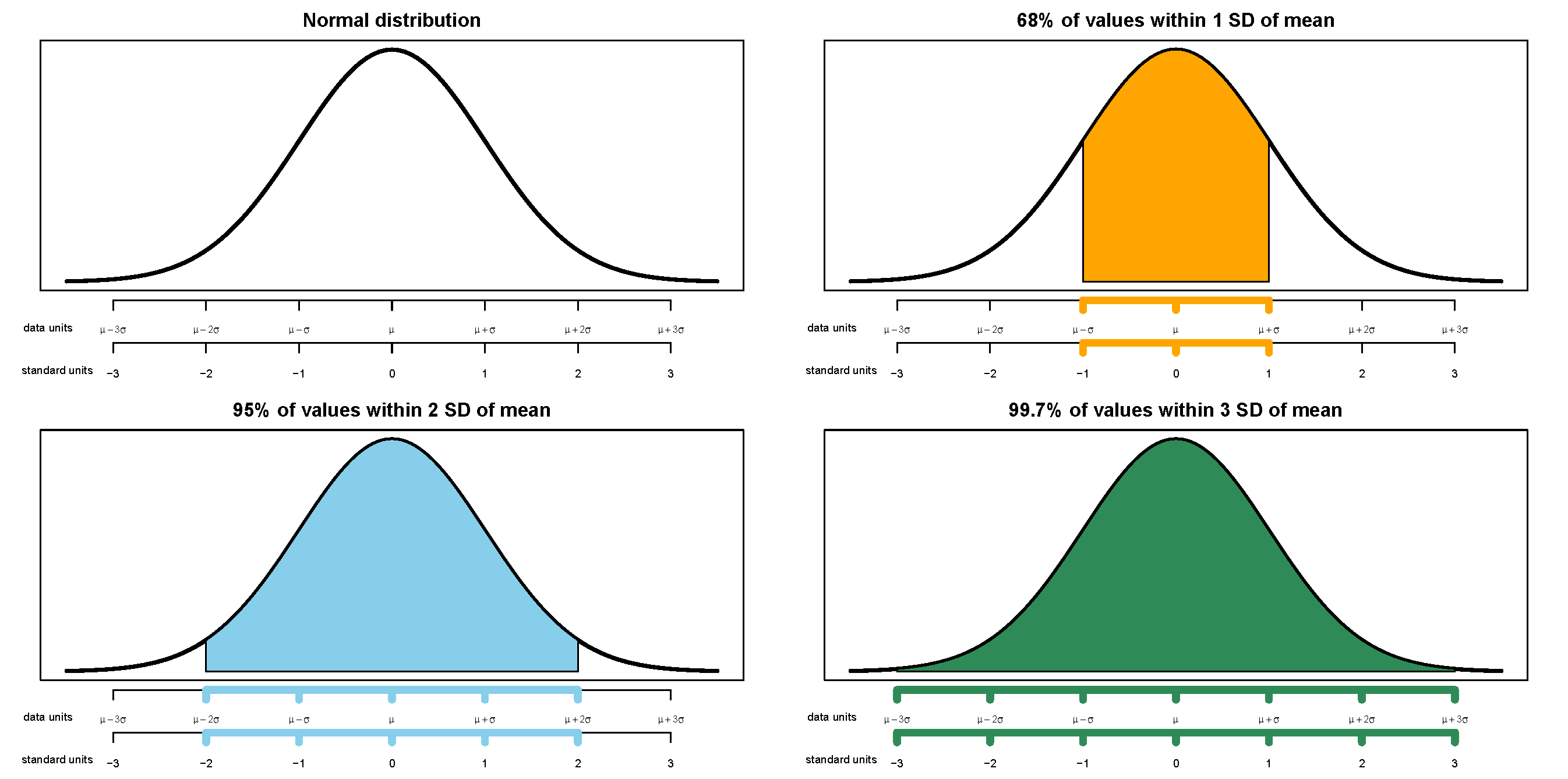
Any Normal distribution follows the “empirical rule” which determines the percentiles that give a Normal distribution its particular bell shape. For example, for any Normal distribution the 84th percentile is about 1 standard deviation above the mean, the 16th percentile is about 1 standard deviation below the mean, and about 68% of values lie within 1 standard deviation of the mean. The table below lists some percentiles of a Normal distribution.
| Percentile | SDs away from the mean |
|---|---|
| 0.1% | 3.09 SDs below the mean |
| 0.5% | 2.58 SDs below the mean |
| 1% | 2.33 SDs below the mean |
| 2.5% | 1.96 SDs below the mean |
| 10% | 1.28 SDs below the mean |
| 15.9% | 1 SDs below the mean |
| 25% | 0.67 SDs below the mean |
| 30.9% | 0.5 SDs below the mean |
| 50% | 0 SDs above the mean |
| 69.1% | 0.5 SDs above the mean |
| 75% | 0.67 SDs above the mean |
| 84.1% | 1 SDs above the mean |
| 90% | 1.28 SDs above the mean |
| 97.5% | 1.96 SDs above the mean |
| 99% | 2.33 SDs above the mean |
| 99.5% | 2.58 SDs above the mean |
| 99.9% | 3.09 SDs above the mean |
The table only lists select percentiles. An even more compact version: For a Normal distribution
- 38% of values are within 0.5 standard deviations of the mean
- 68% of values are within 1 standard deviation of the mean
- 87% of values are within 1.5 standard deviations of the mean
- 95% of values are within 2 standard deviations of the mean
- 99% of values are within 2.6 standard deviations of the mean
- 99.7% of values are within 3 standard deviations of the mean
The “standard” Normal distribution is a Normal(0, 1) distribution, with a mean 0 and a standard deviation of 1. Notice how the empirical rule corresponds to the standard Normal spinner below.
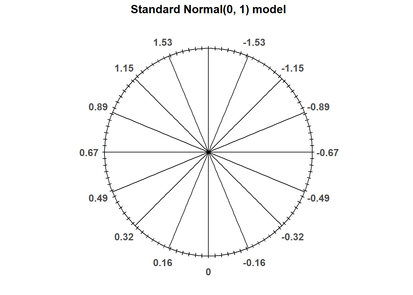
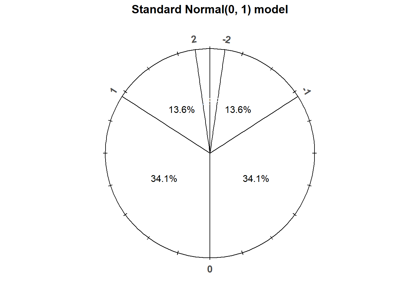
Figure 7.2: A “standard” Normal(0, 1) spinner. The same spinner is displayed on both sides, with different features highlighted on the left and right. Only selected rounded values are displayed, but in the idealized model the spinner is infinitely precise so that any real number is a possible outcome. Notice that the values on the axis are not evenly spaced.
Now we look more closely at where the empirical distribution and the particular bell shape of Normal distributions comes from.
A Normal density is a continuous density on the real line with a particular symmetric “bell” shape. The heart of a Normal density is the function \[ e^{-z^2/2}, \qquad -\infty < z< \infty, \] which defines the general shape of a Normal density. It can be shown that \[ \int_{-\infty}^\infty e^{-z^2/2}dz = \sqrt{2\pi} \] Therefore the function \(e^{-z^2/2}/\sqrt{2\pi}\) integrates to 1.
Definition 7.3 A continuous random variable \(Z\) has a Standard Normal distribution if its pdf140 is \[\begin{align*} \phi(z) & = \frac{1}{\sqrt{2\pi}}\,e^{-z^2/2}, \quad -\infty<z<\infty,\\ & \propto e^{-z^2/2}, \quad -\infty<z<\infty. \end{align*}\]
Z = RV(Normal())

Z.sim(100).plot('rug')
plt.show()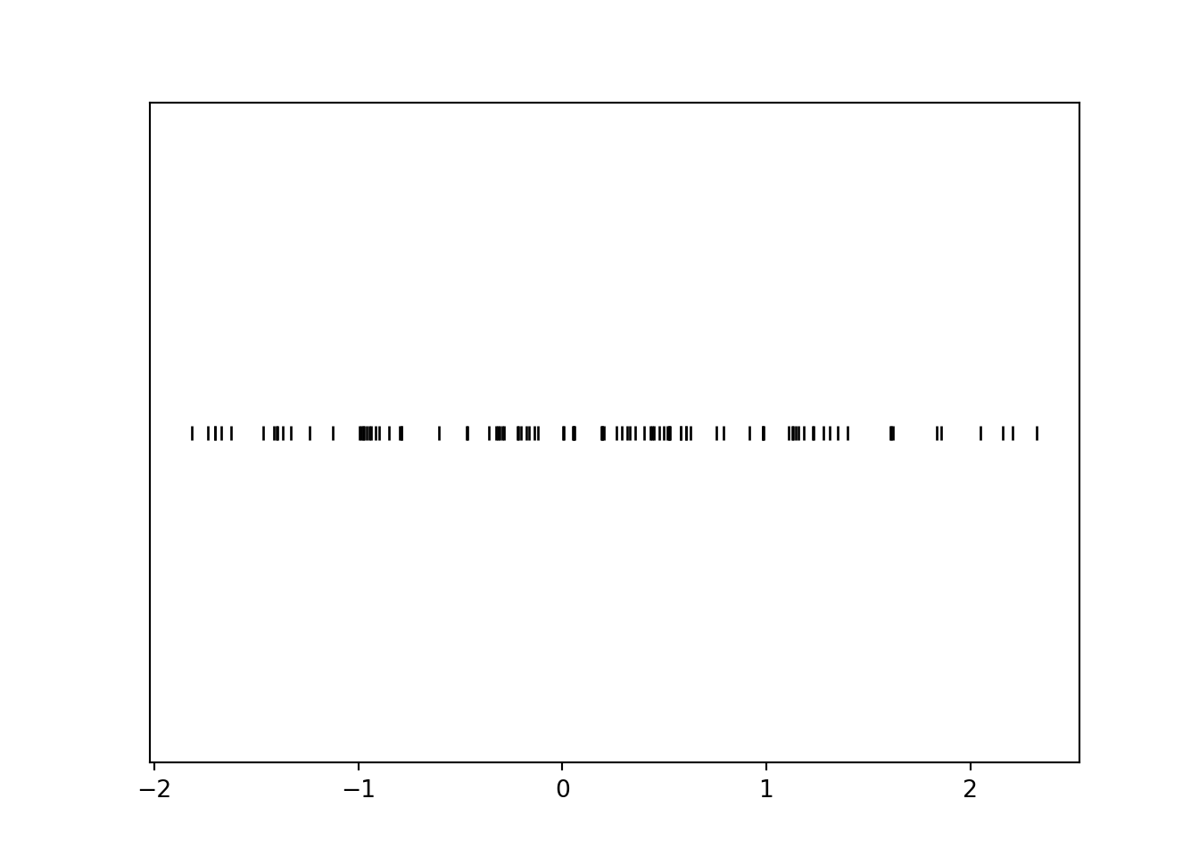
z = Z.sim(10000)

z.plot()

Normal().plot()
plt.show()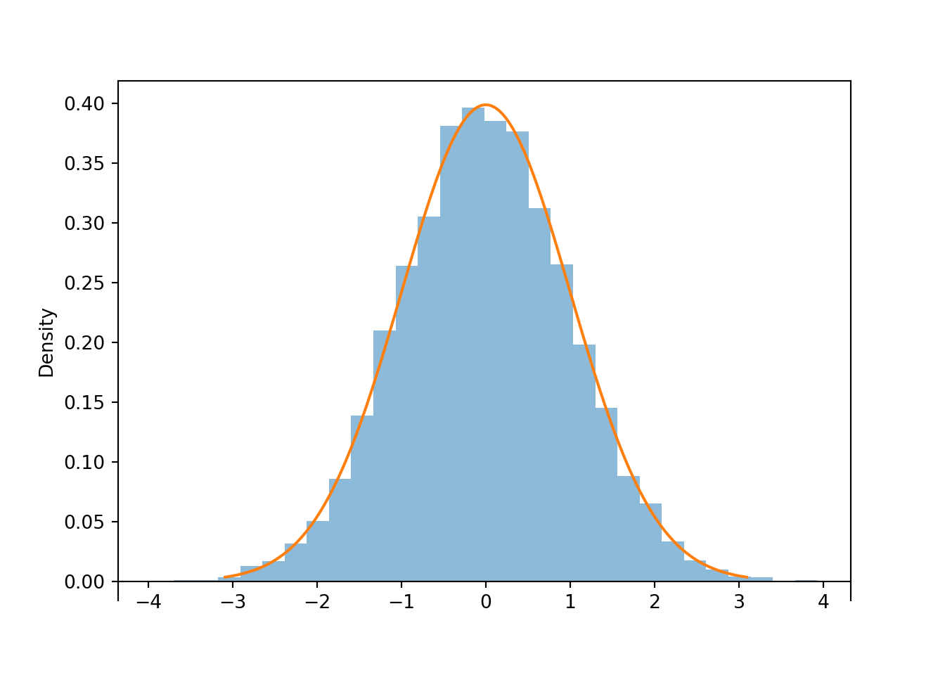
z.mean(), z.sd()## (-0.008990382786713644, 0.9975165149243733)If \(Z\) has a Standard Normal distribution then
\[\begin{align*} \textrm{E}(Z) & = 0\\ \textrm{SD}(Z) & = 1 \end{align*}\]
The Standard Normal pdf is symmetric about its mean of 0, and the peak of the density occurs at 0. The standard deviation is 1, and 1 also indicates the distance from the mean to where the concavity of the density changes. That is, there are inflection points at \(\pm1\).
A random variable with a Standard Normal distribution is in standardized units; the mean is 0 and the standard deviation is 1. We can obtain Normal distribution with other means and standard deviations via linear rescaling. If \(Z\) has a Standard Normal distribution then \(X=\mu + \sigma Z\) has a Normal distribution with mean \(\mu\) and standard deviation \(\sigma\).
Definition 7.4 A continuous random variable \(X\) has a Normal (a.k.a., Gaussian) distribution with mean \(\mu\in (-\infty,\infty)\) and standard deviation \(\sigma>0\) if its pdf is \[\begin{align*} f_X(x) & = \frac{1}{\sigma\sqrt{2\pi}}\,\exp\left(-\frac{1}{2}\left(\frac{x-\mu}{\sigma}\right)^2\right), \quad -\infty<x<\infty,\\ & \propto \exp\left(-\frac{1}{2}\left(\frac{x-\mu}{\sigma}\right)^2\right), \quad -\infty<x<\infty. \end{align*}\]
The Standard Normal distribution is the Normal(0, 1) distribution with mean 0 and standard deviation 1.
If \(X\) has a Normal(\(\mu\), \(\sigma\)) distribution then141 \[\begin{align*} \textrm{E}(X) & = \mu\\ \textrm{SD}(X) & = \sigma \end{align*}\]
A Normal density is a particular “bell-shaped” curve which is symmetric about its mean \(\mu\). The mean \(\mu\) is a location parameter: \(\mu\) indicates where the center and peak of the distribution is.
The standard deviation \(\sigma\) is a scale parameter: \(\sigma\) indicates the distance from the mean to where the concavity of the density changes. That is, there are inflection points at \(\mu\pm \sigma\).
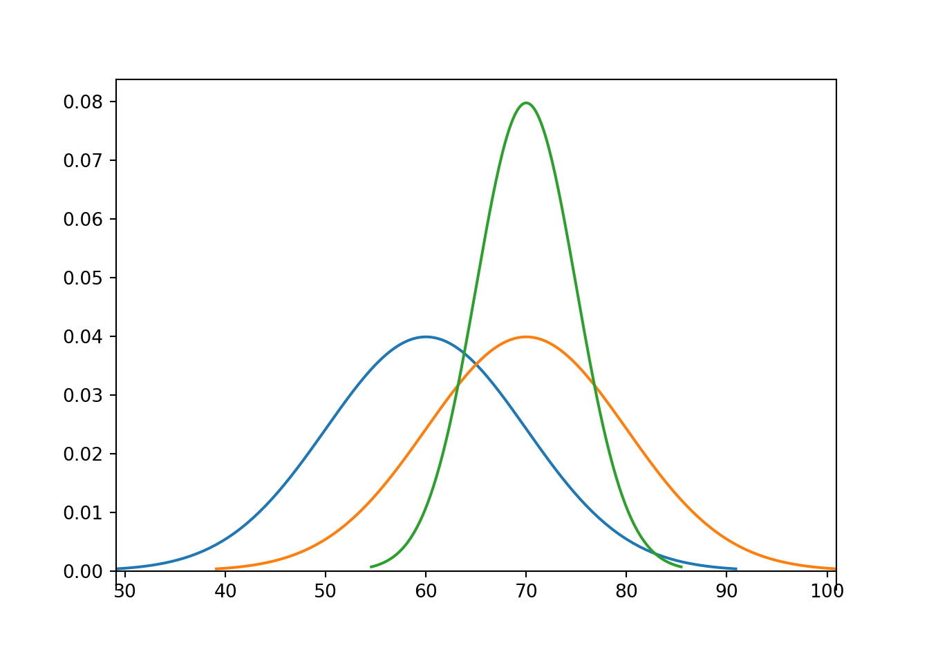
Example 7.8 The pdfs in the plot below represent the distribution of hypothetical test scores in three classes. The test scores in each class follow a Normal distribution. Identify the mean and standard deviation for each class.
Solution. to Example 7.8
Show/hide solution
The blue curve corresponds to a mean of 60; the others to a mean of 70. The green curve corresponds to a standard deviation of 5. Notice that the concavity changes around 65 and 75, so 5 is the distance from the mean to the inflection points. The standard deviation is 10 in the other plots.
If \(Z\) has a Standard Normal distribution its cdf is \[ \Phi(z) = \textrm{P}(Z \le z) = \int_{-\infty}^z \frac{1}{\sqrt{2\pi}}\,e^{-u^2/2}du, \quad -\infty<z<\infty. \] However, there is no closed-form expression for the above integral. The above integral, hence probabilities for a Standard Normal distribution, must be computed through numerical methods.
If \(X\) has a Normal(\(\mu\), \(\sigma\)) distribution then \(X\) has the same distribution as \(\mu + \sigma Z\) where \(Z\) has a Standard Normal distribution, so its cdf is \[ F_X(x) = \textrm{P}(X \le x) = \textrm{P}(\mu + \sigma Z \le x) = \textrm{P}\left(Z \le \frac{x-\mu}{\sigma}\right) = \Phi\left(\frac{x-\mu}{\sigma}\right) \] Therefore, probabilities for any Normal distribution can be found by standardizing and using the Standard Normal cdf, which is basically what we do when we use the “empirical rule”.
Example 7.9 Use the empirical rule to evaluate the following.
- \(\Phi(-1)\)
- \(\Phi(1.5)\)
- \(\Phi^{-1}(0.31)\)
- \(\Phi^{-1}(0.975)\)
Solution. to Example 7.9
Show/hide solution
- \(\Phi(-1)\approx 0.16\). If 68% of values fall in the interval \((-1, 1)\), then 32% fall outside this range, and since the distribution is symmetric, 16% fall in either tail.
- \(\Phi(1.5)\approx 0.935\). If 87% of values fall in the interval \((-1.5, 1.5)\), then 1% fall outside this range, and since the distribution is symmetric, 6.25% fall in either tail.
- \(\Phi^{-1}(0.31)\approx -0.5\). The inverse of the cdf is the quantile function; \(\Phi^{-1}(0.31)\) represents the 31st percentile. Since 38% of values fall in the interval \((-0.5, 0.5)\), then 62% fall outside this range, and since the distribution is symmetric, 31% fall in either tail.
- \(\Phi^{-1}(0.975)\approx 2\). The inverse of the cdf is the quantile function; \(\Phi^{-1}(0.975)\) represents the 97.5th percentile. Since 95% of values fall in the interval \((-2, 2)\), then 5% fall outside this range, and since the distribution is symmetric, 2.5% fall in either tail.
Normal().cdf(-1), Normal().cdf(1.5)## (0.15865525393145707, 0.9331927987311419)
Normal().quantile(0.31), Normal().quantile(0.975)## (-0.4958503473474533, 1.959963984540054)Probabilities and quantiles for Normal distributions can be computed with software. However, you should practice making ballpark estimates without software, by standardizing and using the empirical rule.
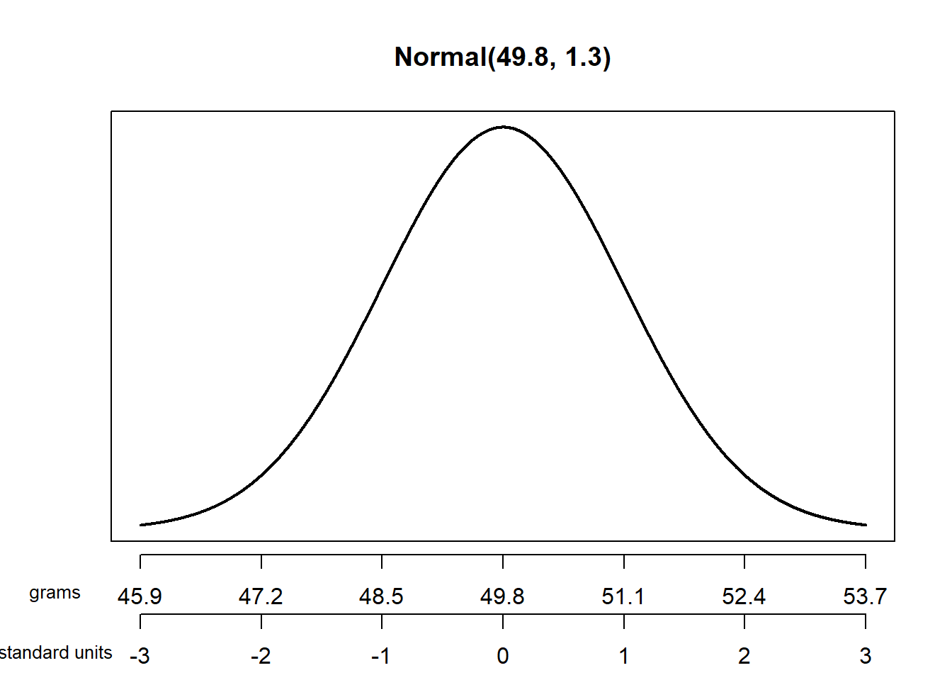
Example 7.10 The wrapper of a package of candy lists a weight of 47.9 grams. Naturally, the weights of individual packages vary somewhat. Suppose package weights have an approximate Normal distribution with a mean of 49.8 grams and a standard deviation of 1.3 grams.
- Sketch the distribution of package weights. Carefully label the variable axis. It is helpful to draw two axes: one in the measurement units of the variable, and one in standardized units.
- Why wouldn’t the company print the mean weight of 49.8 grams as the weight on the package?
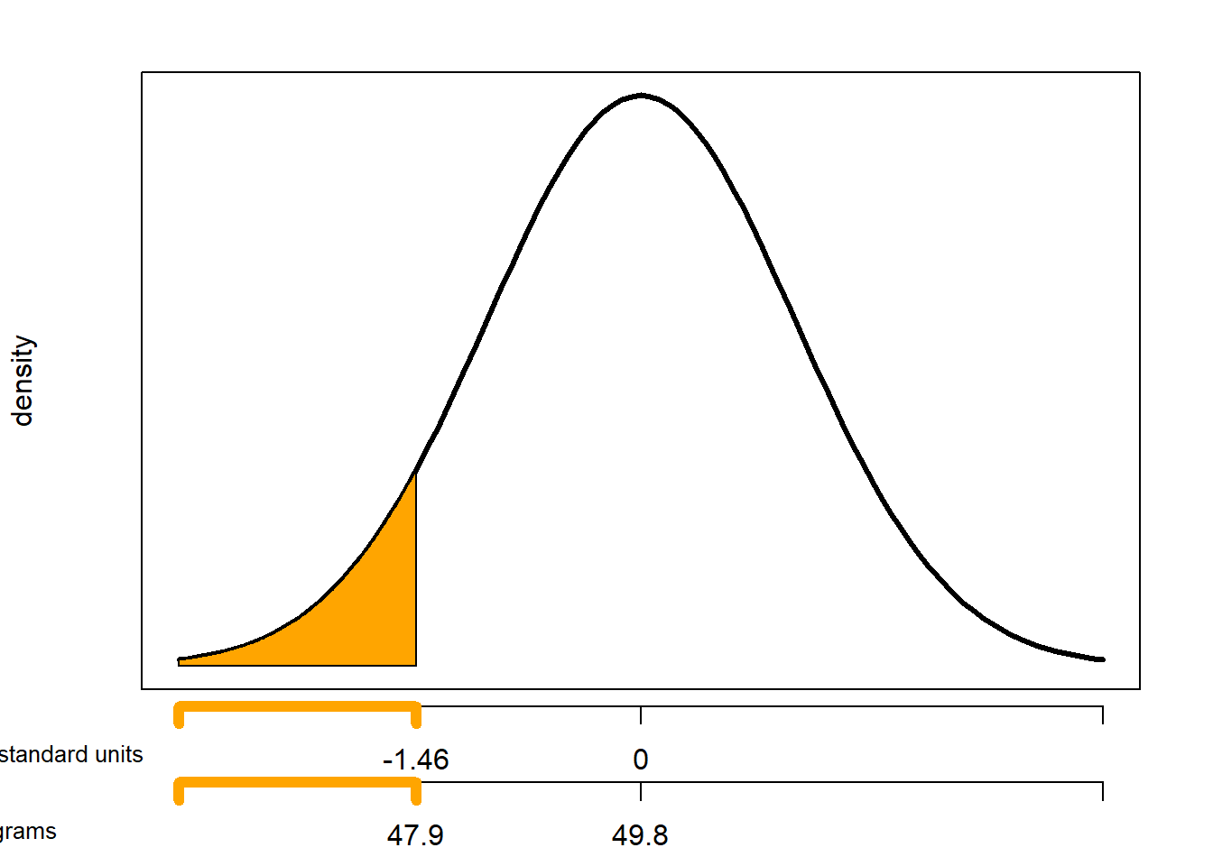
- Estimate the probability that a package weighs less than the printed weight of 47.9 grams.
- Estimate the probability that a package weighs between 47.9 and 53.0 grams.
- Suppose that the company only wants 1% of packages to be underweight. Find the weight that must be printed on the packages.
- Find the 25th percentile (a.k.a., first (lower) quartile) of package weights.
- Find the 75th percentile (a.k.a., third (upper) quartile) of package weights. How can you use the work you did in the previous part?
Solution. to Example 7.10
Show/hide solution
- See the plot below. Be sure to label the variable axis so that the inflection points are 1 SD away from the mean.
- If the company prints the mean weight of 49.8 grams on the package then 50% of the packages would weigh less than the printed weight.
- The standardized value for a weight of 47.9 grams is \((47.9 - 49.8) /1.3=-1.46\). That is, a package weight of 47.9 grams is 1.46 SDs below the mean. From the empirical rule, about 87% of values are within 1.5 SDs of the mean, so 6.5% in either tail. We estimate that the probability is a little larger than 6.5%. Software (below) shows that the probability is 0.072.
- The standardized value for a weight of 53.0 grams is \((53.0 - 49.8) /1.3=-2.46\). That is, a package weight of 53.0 grams is 2.46 SDs above the mean. From the empirical rule, about 99% of values are within 2.6 SDs of the mean, so 0.5% in either tail. Therefore, about 99.5% of packages weigh no more than 53.0 grams. So about \(99.5 - 6.5 = 93\) percent of packages weight between 47.9 and 53.0 grams. Software shows that the probability is 0.921.
- From the empirical rule for 95%, the 2.5th percentile is 2 SDs below the mean. From the empirical rule for 99%, the 0.5th percentile is 2.6 SDs below the mean. So the 1st percentile is between 2 and 2.6 SDs below the mean; software shows that the first percentile is 2.33 SDs below the mean. Therefore, the 1st percentile of package weights is \(49.8 - 2.33\times 1.3 = 46.8\) grams.
- From the empirical rule for 38%, the 31st percentile is 0.5 SDs below the mean. From the empirical rule for 68%, the 16th percentile is 1 SD below the mean. So the 25th percentile is between 0.5 and 1 SDs below the mean; software shows that the 25th percentile is 0.6745 SDs below the mean. Therefore, the 25th percentile of package weights is \(49.8 - 0.6745\times 1.3 = 48.9\) grams.
- By symmetry, if the 25th percentile is 0.6745 SDs below the mean, then the 75th percentile is 0.6745 SDs above the mean. Therefore, the 75th percentile of package weights is \(49.8 + 0.6745\times 1.3 = 50.7\) grams.
Normal(0, 1).cdf((47.9 - 49.8) / 1.3), Normal(49.8, 1.3).cdf(47.9)## (0.07193386424080776, 0.07193386424080776)
Normal(49.8, 1.3).cdf(53.0) - Normal(49.8, 1.3).cdf(47.9)## 0.9211490075663379
Normal(0, 1).quantile(0.01), Normal(49.8, 1.3).quantile(0.01)## (-2.3263478740408408, 46.77574776374691)
Normal(0, 1).quantile(0.25), Normal(0, 1).quantile(0.75)## (-0.6744897501960817, 0.6744897501960817)Standardization is a specific linear rescaling. If \(X\) has a Normal distribution then any linear rescaling of \(X\) also has a Normal distribution. Namely, if \(X\) has a Normal\(\left(\mu,\sigma\right)\) distribution and \(Y=aX+b\) for constants \(a,b\) with \(a\neq 0\), then \(Y\) has a Normal\(\left(a\mu+b, |a|\sigma\right)\) distribution.
Any linear combination of independent Normal random variables has a Normal distribution. If \(X\) and \(Y\) are independent, each with a marginal Normal distribution, and \(a, b\) are non-random constants then \(aX + bY\) has a Normal distribution. (We will see a more general result when we discuss Bivariate Normal distributions.)
Example 7.11 Two people are meeting. (Who? You decide!) Arrival time are measured in minutes after noon, with negative times representing arrivals before noon. Each arrival time follows a Normal distribution with mean 30 and SD 17 minutes, independently of each other.
- Compute the probability that the first person to arrive has to wait more than 15 minutes for the second person to arrive.
- Compute the probability that the first person to arrive arrives before 12:15.
Show/hide solution
- Let \(X, Y\) be the two arrival times, so that \(W=|X-Y|\) is the waiting time. We want \(\text{P}(|X - Y| >15) = \text{P}(X - Y > 15) + \text{P}(X - Y < -15)\). Since \(X\) and \(Y\) are independent each with a Normal distribution, then \(X - Y\) has a Normal distribution; the mean is \(30-30 = 0\), and since \(X\) and \(Y\) are independent \[ \text{Var}(X - Y) = \text{Var}(X) + \text{Var}(V) - 2\text{Cov}(X, Y) = 17^2 + 17^2 - 0 = 578 \] So \(\text{SD}(X - Y) = \sqrt{578} = 24.0\). The standardized value for 15 is \((15 - 0)/24.0=0.624\); that is, 15 is 0.624 SDs above the mean, so \(\textrm{P}(X - Y>15) = 0.266\). Since the distribution of \(X - Y\) is symmetric about 0, \[ \textrm{P}(W > 15) = \textrm{P}(|X-Y|>15) = \textrm{P}(X - Y > 15) + \textrm{P}(X - Y < - 15) = 2(0.266) = 0.53. \] On about 53% of days the first person to arrive has to wait more than 15 minutes for the second to arrive.
- \(T = \min(X, Y)\) is the time at which the first person arrives. The first person arrives before 12:15 if either \(X<15\) or \(Y < 15\), so \(\textrm{P}(T < 15) = \textrm{P}(\{X < 15\}\cup\{Y < 15\})\). It’s easier to compute the probability of the complement. Note that 15 is 0.88 SDs below the mean of \(X\) (\((15 - 30)/17 = -0.88\)) so \(\textrm{P}(X>15) = 0.811\); similarly, \(\textrm{P}(Y > 15) = 0.811\). We want \[\begin{align*} \textrm{P}(T < 15) & = 1 - \textrm{P}(X > 15, Y > 15) && \text{Complement rule}\\ & = 1 - \textrm{P}(X>15)\textrm{P}(Y > 15) && \text{independence of $X, Y$}\\ & = 1- (0.811)(0.811) & & \text{Normal distributions}\\ & = 0.342 \end{align*}\] On about 34% of days the first person arrives before 12:15.
X, Y = RV(Normal(mean = 30, sd = 17) * Normal(mean = 30, sd = 17))

W = abs(X - Y)

T = (X & Y).apply(min)
w = W.sim(10000)
plt.figure()
w.plot()
plt.show()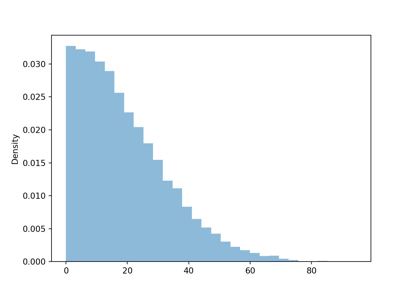
w.mean(), w.sd(), w.count_gt(15) / w.count()## (19.07545240157594, 14.37283042610072, 0.5313)t = T.sim(10000)
plt.figure()
t.plot()
plt.show()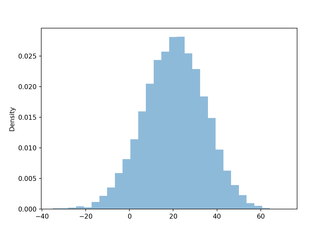
t.mean(), t.sd(), t.count_lt(15) / w.count()## (20.46057657455842, 14.03007165365213, 0.3458)Example 7.12 Daily high temperatures (degrees Fahrenheit) in San Luis Obispo in August follow (approximately) A Normal distribution with a mean of 76.9 degrees F. The temperature exceeds 100 degrees Fahrenheit on about 1.5% of August days.
- What is the standard deviation?
- Suppose the mean increases by 2 degrees Fahrenheit. On what percentage of August days will the daily high temperature exceed 100 degrees Fahrenheit? (Assume the standard deviation does not change.)
- A mean of 78.9 is 1.02 times greater than a mean of 76.9. By what (multiplicative) factor has the percentage of 100-degree days increased? What do you notice?
Show/hide solution
- We are given that 100 is the 98.5th percentile.
Software (
Normal(0, 1).quantile(0.985)) shows that for a Normal distribution the 98.5th percentile is 2.17 standard deviations above the mean. Set \(100 = 76.9 + 2.17\sigma\) and solve for the standard deviation \(\sigma = 10.65\) degrees F. - The mean is now 78.9. Now the value 100 is \((100-78.9)/10.65 = 1.98\) standard deviations above the mean.
Software (
1 - Normal(0, 1).cdf(1.98)) shows that for a Normal distribution the probability of a value more than 1.98 standard deviations above the mean is 0.023. On 2.3% of August days the daily high temperature will exceed 100 degrees F. - \(0.023/0.015 = 1.53\). A 2 percent increase in the mean results in a 53 percent increase in the probability that a day has a daily high temperature above 100 degrees F. Relative small changes in the mean can have relative large impacts on tail probabilities.
Example 7.13 In a large class, scores on midterm 1 follow (approximately) a Normal\((\mu_1, \sigma)\) distribution and scores on midterm 2 follow (approximately) a Normal\((\mu_2, \sigma)\) distribution. Note that the SD \(\sigma\) is the same on both exams. The 40th percentile of midterm 1 scores is equal to the 70th percentile of midterm 2 scores. Compute \[ \frac{\mu_1-\mu_2}{\sigma} \] (This is one statistical measure of effect size.)
Show/hide solution
Software shows that for a Normal distribution, the 40th percentile is 0.253 SDs below the mean and the 70th percentile is 0.524 SDs above the mean. The 40th percentile of midterm 1 scores is \(\mu_1 - 0.253 \sigma\), and the 70th percentile of midterm 2 scores is \(\mu_2 + 0.524\sigma\). We are told \[ \mu_1 - 0.253 \sigma = \mu_2 + 0.524\sigma \] Solve for \[ \frac{\mu_1-\mu_2}{\sigma} = 0.524 + 0.253 = 0.78 \] The effect size is 0.78. The mean on midterm 1 is 0.78 SDs above the mean on midterm 2.
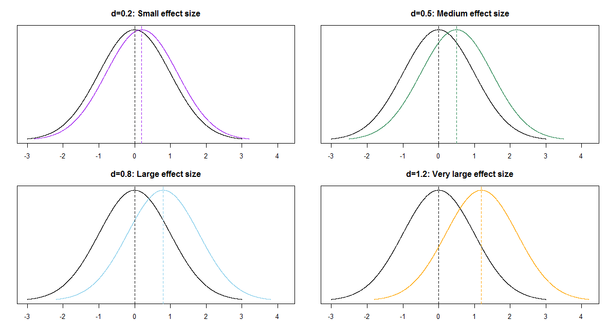
The previous example illustrates a common problem in statistics: comparing two (or more) groups; in particular, comparing two means. When comparing groups, a more important question than “is there a difference?” is “how large is the difference?” An effect size is a measure of the magnitude of a difference between groups. When comparing a numerical variable between two groups, one measure of the population effect size is Cohens’s \(d\) \[ \frac{\mu_1 - \mu_2}{\sigma} \]
The values of any numerical variable vary naturally from unit to unit. The SD of the numerical variable measures the degree to which individual values of the variable vary naturally, so the SD provides a natural “scale” for the variable. Cohen’s \(d\) compares the magnitude of the difference in means relative to the natural scale (SD) for the variable
Some rough guidelines for interpreting \(|d|\):
| d | 0.2 | 0.5 | 0.8 | 1.2 | 2.0 |
| Effect size | Small | Medium | Large | Very Large | Huge |
For example, assume the two population distributions are Normal and the two population standard deviations are equal. Then when the effect size is 1.0 the median of the distribution with the higher mean is the 84th percentile of the distribution with the lower mean, which is a very large difference.
| d | 0.2 | 0.5 | 0.8 | 1.0 | 1.2 | 2.0 |
| Effect size | Small | Medium | Large | Very Large | Huge | |
| Median of population 1 is | ||||||
| (blank) percentile of population 2 | 58th | 69th | 79th | 84th | 89th | 98th |
The Standard Normal pdf is typically denoted \(\phi(\cdot)\), the lowercase Greek letter “phi”, and the cdf is denoted \(\Phi(\cdot)\), the uppercase Greek letter “phi”.↩︎
If we write \(N(0, 4)\) we mean a Normal distribution with mean 0 and standard deviation 4. Be aware that some references refer to a Normal distribution by its mean and variance, in which case \(N(0, 4)\) would refer to a Normal distribution with mean 0 and variance 4.↩︎