7.3 Bivariate Normal distributions
Just as Normal distributions are the most important univariate distributions, joint or multivariate Normal distributions are the most important joint distributions. We mostly focus on the case of two random variables.
Jointly continuous random variables \(X\) and \(Y\) have a Bivariate Normal distribution with parameters \(\mu_X\), \(\mu_Y\), \(\sigma_X>0\), \(\sigma_Y>0\), and \(-1<\rho<1\) if the joint pdf is
{ \[\begin{align*} f_{X, Y}(x,y) & = \frac{1}{2\pi\sigma_X\sigma_Y\sqrt{1-\rho^2}}\exp\left(-\frac{1}{2(1-\rho^2)}\left[\left(\frac{x-\mu_X}{\sigma_X}\right)^2+\left(\frac{y-\mu_Y}{\sigma_Y}\right)^2-2\rho\left(\frac{x-\mu_X}{\sigma_X}\right)\left(\frac{y-\mu_Y}{\sigma_Y}\right)\right]\right), \quad -\infty <x<\infty, -\infty<y<\infty \end{align*}\] }
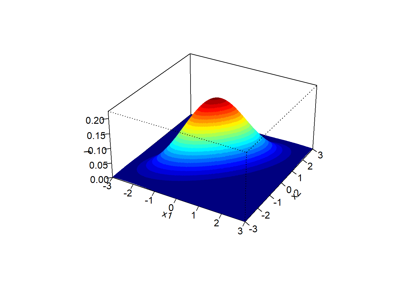
It can be shown that if the pair \((X, Y)\) has a BivariateNormal(\(\mu_X\), \(\mu_Y\), \(\sigma_X\), \(\sigma_Y\), \(\rho\)) distribution \[\begin{align*} \textrm{E}(X) & =\mu_X\\ \textrm{E}(Y) & =\mu_Y\\ \textrm{SD}(X) & = \sigma_X\\ \textrm{SD}(Y) & = \sigma_Y\\ \textrm{Corr}(X, Y) & = \rho \end{align*}\] A Bivariate Normal pdf is a density on \((x, y)\) pairs. The density surface looks like a mound with a peak at the point of means \((\mu_X,\mu_Y)\).
A Bivariate Normal Density has elliptical contours. For each height \(c>0\) the set \(\{(x,y): f_{X, Y}(x,y)=c\}\) is an ellipse. The density decreases as \((x, y)\) moves away from \((\mu_X, \mu_Y)\), most steeply along the minor axis of the ellipse, and least steeply along the major of the ellipse.
A scatterplot of \((x,y)\) pairs generated from a Bivariate Normal distribution will have a rough linear association and the cloud of points will resemble an ellipse.
X,Y = RV(BivariateNormal(mean1 = 0, mean2 = 0, sd1 = 1, sd2 = 1, corr = -0.5))
(X & Y).sim(1000).plot(['scatter', 'marginal'])
plt.show()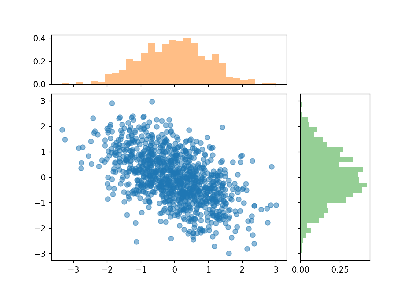
If \(X\) and \(Y\) have a Bivariate Normal distribution, then the marginal distributions are also Normal: \(X\) has a Normal\(\left(\mu_X,\sigma_X\right)\) distribution and \(Y\) has a Normal\(\left(\mu_Y,\sigma_Y\right)\).
The strength of the association in a Bivariate Normal distribution is completely determined by the correlation \(\rho\). Remember, in general it is possible to have situations where the correlation is 0 but the random variables are not independent. However, for Bivariate Normal distributions independence and uncorrelatedness are equivalent.
Theorem 7.1 If \(X\) and \(Y\) have a Bivariate Normal distribution and \(\textrm{Corr}(X, Y)=0\) then \(X\) and \(Y\) are independent.
The above is true because the joint pdf factors into the product of the marginal pdfs if and only if \(\rho=0\).
It can also be shown that if \(X\) and \(Y\) have a Bivariate Normal distribution then any conditional distribution is Normal. The conditional distribution of \(Y\) given \(X=x\) is \[ N\left(\mu_Y + \frac{\rho\sigma_Y}{\sigma_X}\left(x-\mu_X\right),\;\sigma_Y\sqrt{1-\rho^2}\right) \]
(Y | (abs(X - 1.5) < 0.1) ).sim(1000).plot()
(Y | (abs(X - (-0.5)) < 0.1) ).sim(1000).plot()
plt.show()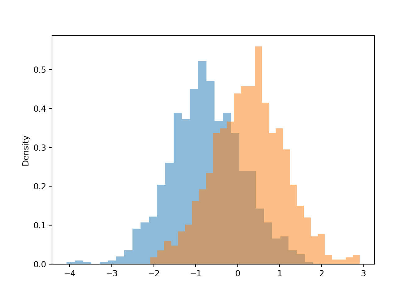
The conditional expected value of \(Y\) given \(X=x\) is a linear function of \(x\), called the regression line of \(Y\) on \(X\): \[ \textrm{E}(Y | X=x) = \mu_Y + \rho\sigma_Y\left(\frac{x-\mu_X}{\sigma_X}\right) \] The regression line passes through the point of means \((\mu_X, \mu_Y)\) and has slope \[ \frac{\rho \sigma_Y}{\sigma_X} \] The regression line estimates that if the given \(x\) value is \(z\) SDs above of the mean of \(X\), then the corresponding \(Y\) values will be, on average, \(\rho z\) SDs away from the mean of \(Y\) \[ \frac{\textrm{E}(Y|X=x) - \mu_Y}{\sigma_Y} = \rho\left(\frac{x-\mu_X}{\sigma_X}\right) \] Since \(|\rho|\le 1\), for a given \(x\) value the corresponding \(Y\) values will be, on average, relatively closer to the mean of \(Y\) than the given \(x\) value is to the mean of \(X\). This is known as regression to the mean.
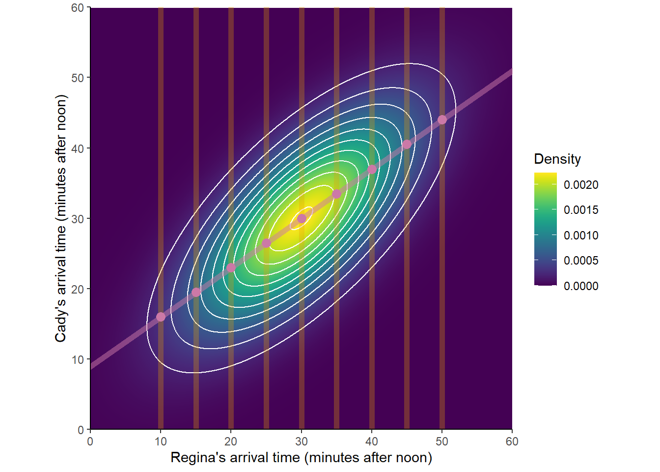
Figure 7.3: A Bivariate Normal distribution with some conditional distributions and conditional expected values highlighted.
For Bivariate Normal distributions, the conditional variance of \(Y\) given \(X=x\) does not depend on \(x\): \[ \textrm{SD}(Y |X = x) = \sigma_Y\sqrt{1-\rho^2} \] The \(Y\) values corresponding to a particular \(x\) value are less variable then the entire collection of \(Y\) values.
Theorem 7.2 \(X\) and \(Y\) have a Bivariate Normal distribution if and only if every linear combination of \(X\) and \(Y\) has a Normal distribution. That is, \(X\) and \(Y\) have a Bivariate Normal distribution if and only if \(aX+bY+c\) has a Normal distribution for all142 \(a\), \(b\), \(c\).
(X + Y).sim(10000).plot()
plt.show()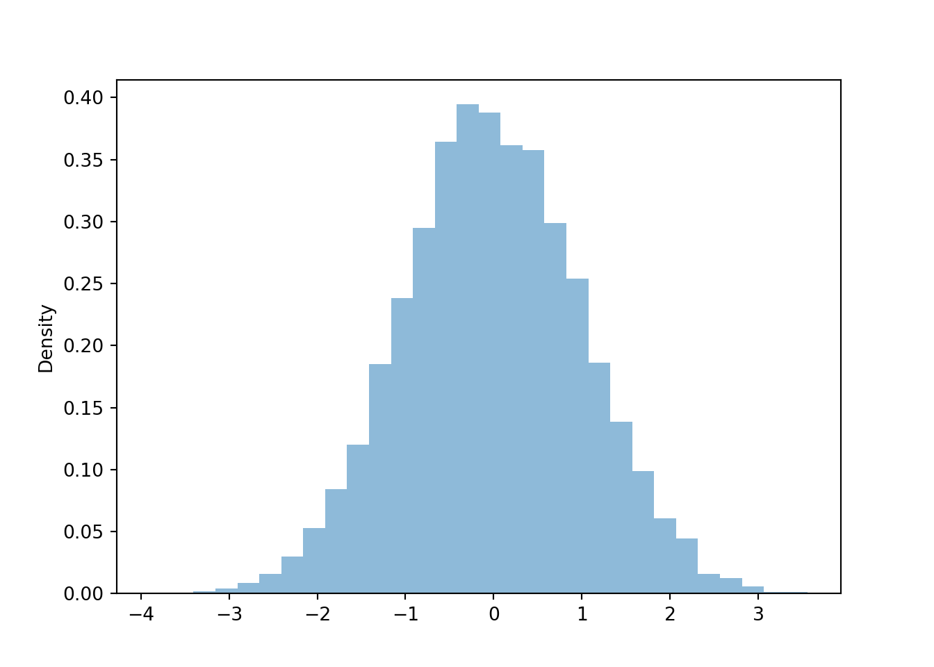
In short, if \(X\) and \(Y\) have a Bivariate Normal distribution then “everything is Normal”: marginal distributions are Normal, conditional distributions are Normal, and distributions of linear combinations are Normal. Therefore, probabilities for Bivariate Normal distribution problems can be solved by identifying the proper Normal distribution — that is, its mean and variance — standardizing, and using the empirical rule.
Example 7.14 Suppose that SAT Math (\(M\)) and Reading (\(R\)) scores of CalPoly students have a Bivariate Normal distribution. Math scores have mean 640 and SD 80, Reading scores have mean 610 and SD 70, and the correlation between scores is 0.7.
- Find the probability that a student has a Math score above 700.
- Find the probability that a student has a total score above 1500.
- Compute and interpret \(\textrm{E}(M|R = 700)\).
- Find the probability that a student has a higher Math than Reading score if the student scores 700 on Reading.
- Describe how you could use a Normal(0, 1) spinner to simulate an \((X, Y)\) pair.
- Find the probability that a student has a higher Math than Reading score.
Show/hide solution
- Find the probability that a student has a Math score above 700. Math score \(M\) has a Normal(640, 80) distribution. A Math score of 700 is \((700-640)/80=0.75\) SDs above the mean Math score. The probability is \(\textrm{P}(M > 700) = 1-\Phi(0.75)\approx 0.227\).
- Find the probability that a student has a total score above 1500. Total score \(T=M+R\) has a Normal distribution with mean \(\textrm{E}(T)=\textrm{E}(M)+\textrm{E}(R) = 640 + 610 = 1250\). The variance is \[\begin{align*} \textrm{Var}(M+R) & = \textrm{Var}(M) + \textrm{Var}(R) + 2\textrm{Cov}(M, R)\\ & = 80^2 + 70^2 + 2(0.7)(80)(70) = 19140 \end{align*}\] The SD is 138. Therefore we want to find \(\textrm{P}(T > 1500)\) where \(T\) has a Normal(1250, 138) distribution. With respect to this distribution, a total score of 1500 is \((1500-1250)/138 = 1.81\) SDs above the mean so \(\textrm{P}(T >1500) = 1 - \Phi(1.81)\approx 0.035\).
- Compute and interpret \(\textrm{E}(M|R = 700)\). A Reading score of 700 is \((700-610)/70=1.29\) SDs above the mean Reading score. The correlation is 0.7, so we expect the Math score to be \((0.7)(1.29)=0.9\) SDs above the mean Math score, so \(\textrm{E}(M|R = 700) = 640 + 0.9(80) = 712\). Among students who score a 700 on Reading the average Math score is 712.
- Find the probability that a student has a higher Math than Reading score if the student scores 700 on Reading. We want \(\textrm{P}(M > R|R = 700) = \textrm{P}(M > 700 | R = 700)\). The conditional distribution of \(M\) given \(R=700\) is Normal with mean 712 and SD \(80\sqrt{1-0.7^2} = 57.1\). With respect to this distribution, a M score of 700 is \((700-712)/57.1=-0.2\), that is 0.2 SDs below the conditional mean Math score. The probability that we want is \(\textrm{P}(M > 700 | R = 700) = 1 - \Phi(-0.21) =0.583\).
- Spin the Normal(0, 1) spinner to generate \(Z_1\) and let \(R = 610 + 70Z_1\). For any \(R\), the conditional SD of \(M\) given \(R\) is \(80\sqrt{1-0.7^2} = 57.1\). Given \(R\) find the conditional mean of \(M\), \(\mu_{M|R}\). For example, if \(R=700\) then the conditional mean of \(M\) is \(\mu_{M|R=700}=712\). Spin the Normal(0, 1) spinner again to generate \(Z_2\) and let \(M=\mu_{M|R} + 57.1Z_2\).
- Find the probability that a student has a higher Math than Reading score. We want \(\textrm{P}(M > R)\). The key is to write this probability in terms of a linear combination: \(\textrm{P}(M >R) = \textrm{P}(M - R > 0)\). The linear combination \(M-R\) has a Normal distribution with mean \(\textrm{E}(M-R)=\textrm{E}(M)-\textrm{E}(R) = 640 - 610 = 30\) and variance \[\begin{align*} \textrm{Var}(M-R) & = \textrm{Var}(M) + \textrm{Var}(R) - 2\textrm{Cov}(M, R)\\ & = 80^2 + 70^2 - 2(0.7)(80)(70) = 3460 \end{align*}\] The SD is 58.8. Therefore we want to find \(\textrm{P}(D > 0)\) where \(D=M-R\) has a Normal(30, 58.8) distribution. With respect to this distribution, a difference of 0 is \((0-30)/58.8 = -0.51\), that is 0.51 SDs below the mean so \(\textrm{P}(D >0) = 1 - \Phi(-0.51)\approx 0.695\).
M, R = RV(BivariateNormal(mean1 = 640, sd1 = 80, mean2 = 610, sd2 = 70, corr = 0.7))
(M & R).sim(1000).plot()
plt.show()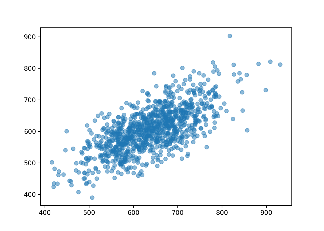
You might think that if both \(X\) and \(Y\) have Normal distributions then their joint distribution is Bivariate Normal. But this is not true in general, as the following example shows. This is a particular example of a general concept we have seen often: marginal distributions alone are not enough to specify the joint distribution (unless the random variables are independent).
Example 7.15 Let \(X\) and \(I\) be independent, \(X\) has a Normal(0,1) distribution, and \(I\) takes values 1 or \(-1\) with probability \(1/2\) each. Let \(Y=IX\).
- How could you use spinners to simulate an \((X, Y)\) pair?
- Identify the distribution of \(Y\).
- Sketch a scatterplot of simulated \((X, Y)\) values.
- Are \(X\) and \(Y\) independent? (Careful, it is not enough to say “no, because \(Y\) is a function of \(X\)”. You can check that \(Y\) and \(I\) are independent even though \(Y\) is a function of \(I\).)
- Find \(\textrm{Cov}(X,Y)\) and \(\textrm{Corr}(X,Y)\).
- Is the distribution of \(X+Y\) Normal? (Hint: find \(\textrm{P}(X+Y=0)\).)
- Does the pair \((X, Y)\) have a Bivariate Normal distribution?
Show/hide solution
- \(I\) can be determined by a coin flip; \(I=1\) if the flip lands on Heads, \(I=-1\) if the flip lands on Tails. Spin the Normal(0, 1) spinner to generate \(Z\) and flip the coin; if it lands Heads then \(Y=Z\), if Tails then \(Y=-Z\).
- The conditional distribution of \(Y\) given \(I=1\) is Normal(0, 1) since in this case \(Y=Z\). The conditional distribution of \(Y\) given \(I=-1\) is Normal(0, 1) since in this case \(Y=-Z\), and the Normal(0, 1) distribution is symmetric about 0.
- Half of the \((X, Y)\) pairs lie on the line \(y=x\) and the other half on the line \(y=-x\). So the scatter plot looks like an “X”.
- \(X\) and \(Y\) are not independent. The marginal distribution of \(Y\) is Normal(0, 1), but conditional on \(X=1\), \(Y\) only takes value 1 or \(-1\) with probability 1/2 each.
- Conditional \(X=x\), \(Y\) only takes value \(x\) or \(-x\) with probability 1/2 each, so \(\textrm{E}(Y|X)=0\). Therefore, \(\textrm{Cov}(X, Y) = 0\). \(X\) and \(Y\) are uncorrelated.
- \(X+Y\) does not have a continuous distribution. \(\textrm{P}(X + Y = 0) = \textrm{P}(Y = -X) = \textrm{P}(I=-1)=1/2\neq 0\). If \(X+Y\) had a Normal distribution then \(\textrm{P}(X+Y=0)\) would be 0 because a Normal distribution is a continuous distribution. (The random variable \(X+Y\) is neither discrete nor continuous.)
- Even though each of \(X\) and \(Y\) has a Normal distribution, the pair \((X, Y)\) does not have a Bivariate Normal distribution.
- The scatterplot of \((X, Y)\) pairs is not elliptical.
- \(X\) and \(Y\) are uncorrelated but not independent.
- The conditional distribution of \(Y\) given \(X=x\) is not Normal.
- The linear combination \(X+Y\) does not have a Normal distribution.
If the pair \((X,Y)\) has a joint Normal distribution then each of \(X\) and \(Y\) has a Normal distribution. But the example shows that the converse is not true. That is, if each of \(X\) and \(Y\) has a Normal distribution, it is not necessarily true that the pair \((X, Y)\) has a joint Normal distribution
However, if \(X\) and \(Y\) are independent and each of \(X\) and \(Y\) has a Normal distribution, then the pair \((X, Y)\) has a joint Normal distribution.
The following is a standardization result for which can be used to simulate values from a Bivariate Normal distribution.
Let \(Z_1, Z_2\) be independent, each having a Normal(0, 1) distribution. For constants \(\mu_X\), \(\mu_Y\), \(\sigma_X\), \(\sigma_Y\), and \(-1<\rho<1\) define \[\begin{align*} X & = \mu_X + \sigma_X Z_1\\ Y & = \mu_Y + \rho\sigma_Y Z_1 + \sqrt{1-\rho^2}\, \sigma_Y Z_2. \end{align*}\] Then the pair \((X,Y)\) has a BivariateNormal(\(\mu_X,\mu_Y,\sigma_X,\sigma_Y,\rho)\) distribution.
Random variables \(X_1, \ldots, X_n\) have a Multivariate Normal (MVN) (a.k.a., joint Gaussian) distribution if and only if for all non-random constants \(a_1,\ldots,a_n\), the RV \(a_1X_1+\cdots+a_n X_n\) has a Normal distribution. That is, if random variables have a MVN distribution then any random variable formed by taking a linear combination of the RVs has a Normal distribution. In particular, each \(X_i\) must have a marginal Normal distribution.
In fact, a more general result is true: any random vector whose components are formed by taking linear combinations of a MVN random vector is itself a MVN random vector. As a special case, if \(X_1,\ldots, X_n\) are independent and each \(X_i\) has a Normal distribution, then their joint distribution is MVN.
If random variables \(X_1,\ldots, X_n\) have a Multivariate Normal distribution, then their joint distribution is fully specified by
- the mean vector, with entries \(\textrm{E}(X_i)\), \(i=1,\ldots,n\)
- the covariance matrix, with entries \(\textrm{Cov}(X_i,X_j)\), \(i,j=1,\ldots, n\)
Random variables \(X\) and \(Y\) which have a MVN distribution are independent if and only if \(\textrm{Cov}(X,Y)=0\).
At least one of \(a\), \(b\) must not be 0, unless degenerate Normal distributions are considered. A non-random constant \(c\) can be considered a degenerate Normal random variable with a mean of \(c\) and a SD of 0.↩︎