2.9 Averages
On any single repetition of the simulation a particular event either occurs or not. Summarizing simulation results for events involves simply counting the number of repetitions on which the event occurs and finding related proportions.
On the other hand, random variables typically take many possible values over the course of many repetitions. We are still interested in relative frequencies of events, like \(\{X=6\}\), \(\{Y \ge 3\}\), and \(\{X > 5, Y \ge 3\}\). But for random variables we are also interested in their distributions which describe the possible values that the random variables can take and their relative likelihoods. While the marginal distribution contain all the information about a single random variables, it is also useful to summarize some key features of a distribution. For example, probabilities of particular events concerning a random variable can be interpreted as long run relative frequencies.
One summary characteristic of a distribution is the long run average value of the random variable. We can approximate the long run average value by simulating many values of the random variable and computing the average (mean) in the usual way.
Example 2.48 Let \(X\) be the sum of two rolls of a fair four-sided die, and let \(Y\) be the larger of the two rolls (or the common value if a tie). Recall your tactile simulation from Example 2.29. Based only on the results of your simulation, approximate the long run average value of each of the following. (Don’t worry if the approximations are any good yet.)
- \(X\)
- \(Y\)
- \(X^2\)
- \(XY\)
Solution. to Example 2.48.
Our simulation results are in Table 2.23 below.
- Approximate the long run average value of \(X\) by summing the 10 simulated values of \(X\) and dividing by 10. \[ \frac{3 + 2 + 6 + 7 + 5 + 7 + 5 + 6 + 3 + 7}{10} = 5.1 \]
- Approximate the long run average value of \(Y\) by summing the 10 simulated values of \(Y\) and dividing by 10. \[ \frac{2 + 1 + 3 + 4 + 3 + 4 + 3 + 4 + 2 + 4}{10} = 3 \]
- First, for each repetition square the value of \(X\) to obtain the \(X^2\) column. Then approximate the long run average value of \(X^2\) by summing the 10 simulated values of \(X^2\) and dividing by 10. \[ \frac{9 + 4 + 36 + 49 + 25 + 49 + 25 + 36 + 9 + 49}{10} = 29.1 \]
- First, for each repetition compute the product \(XY\) to obtain the \(XY\) column. Then approximate the long run average value of \(XY\) by summing the 10 simulated values of \(XY\) and dividing by 10. \[ \frac{6 + 2 + 18 + 28 + 15 + 28 + 15 + 24 + 6 + 28}{10} = 17 \]
We reproduce the results of our simulation in Table 2.23 with additional columns for \(X^2\) and \(XY\). Results vary naturally so your simulation results will be different, but the same ideas apply.
| Repetition | First roll | Second roll | X | Y | X^2 | XY |
|---|---|---|---|---|---|---|
| 1 | 2 | 1 | 3 | 2 | 9 | 6 |
| 2 | 1 | 1 | 2 | 1 | 4 | 2 |
| 3 | 3 | 3 | 6 | 3 | 36 | 18 |
| 4 | 4 | 3 | 7 | 4 | 49 | 28 |
| 5 | 3 | 2 | 5 | 3 | 25 | 15 |
| 6 | 3 | 4 | 7 | 4 | 49 | 28 |
| 7 | 2 | 3 | 5 | 3 | 25 | 15 |
| 8 | 2 | 4 | 6 | 4 | 36 | 24 |
| 9 | 1 | 2 | 3 | 2 | 9 | 6 |
| 10 | 3 | 4 | 7 | 4 | 49 | 28 |
Of course, 10 repetitions is not enough to reliably approximate the long run average value. But whether the average is based on 10 values or 10 million, an average is computed in the usual way: sum the values and divide by the number of values. We’ll consider what happens in the long run soon, but first a caution about averages of transformations.
Example 2.49 Donny Don’t says: “Why bother creating columns for \(X^2\) and \(XY\)? If I want to find the average value of \(X^2\) I can just square the average value of \(X\). For the average value of \(XY\) I can just multiply the average value of \(X\) and the average value of \(Y\).” Do you agree? (Check to see if this works for your simulation results.) If not, explain why not.
Solution. to Example 2.49
It is easy to check that Donny is wrong just by inspecting the simulation results: 5.12 \(\neq\) 29.1, 5.1 \(\times\) 3 \(\neq\) 17. To see why, suppose we had just performed two repetitions, resulting in the first two rows of Table 2.23. \[ \text{Average of $X^2$} = \frac{3^2 + 2^2}{2} =6.5 \neq 6.25= \left(\frac{3 + 2}{2}\right)^2=(\text{Average of $X$})^2 \] Squaring first and then averaging (which yields 6.5) is not the same as averaging first and then squaring (which yields 6.25), essentially because \((3+2)^2\neq 3^2 + 2^2\).
Similarly, \[ {\small \text{Average of $XY$} = \frac{(3)(2) + (2)(1)}{2} =4 \neq 3.75= \left(\frac{3 + 2}{2}\right)\left(\frac{2 + 1}{2}\right)=(\text{Average of $X$})\times (\text{Average of $Y$}) } \] Multiplying first and then averaging (which yields 4) is not the same as averaging first and then multiplying (which yields 3.75), essentially because \((3)(2)+(2)(1)\neq(3+2)(2+1)\).
In general the order of transforming and averaging is not interchangeable. Whether in the short run or the long run, in general \[ \begin{align*} \text{Average of $g(X)$} & \neq g(\text{Average of $X$})\\ \text{Average of $g(X, Y)$} & \neq g(\text{Average of $X$}, \text{Average of $Y$}) \end{align*} \] Many common mistakes in probability result from not heeding this principle, so we will introduce many related examples to help you practice your understanding.
2.9.1 Long run averages
Now let’s see what happens in the long run. Let \(X\) be the sum of two rolls of a fair four-sided die. Table 2.24 displays the results of 10 pairs of rolls of a fair four-sided die. The first column is the repetition number (first pair, second pair, and so on) and the second column represents \(X\), the sum of the two rolls. The third column displays the running sum of \(X\) values, and the fourth column the running average of \(X\) values. Of course, the results depend on the particular sequence of rolls. We encourage you to roll the dice and compare your results.
| Repetition | Value of X | Running sum of X | Running average of X |
|---|---|---|---|
| 1 | 3 | 3 | 3.000 |
| 2 | 2 | 5 | 2.500 |
| 3 | 6 | 11 | 3.667 |
| 4 | 7 | 18 | 4.500 |
| 5 | 5 | 23 | 4.600 |
| 6 | 7 | 30 | 5.000 |
| 7 | 5 | 35 | 5.000 |
| 8 | 6 | 41 | 5.125 |
| 9 | 3 | 44 | 4.889 |
| 10 | 7 | 51 | 5.100 |
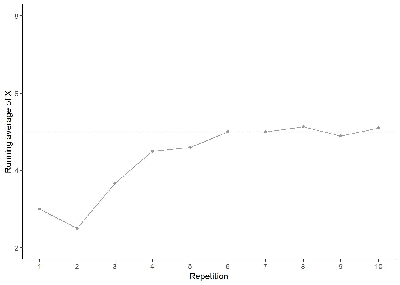
Figure 2.34: Running average of \(X\) for the 10 pairs of rolls in Table 2.24.
Now we’ll perform 90 more repetitions for a total of 100. The plot on the left in Figure 2.35 summarizes the results, while the plot on the right also displays the results for 3 additional sets of 100 pairs of rolls. The running average fluctuates considerably in the early stages, but settles down and tends to get closer to 5 as the number of flips increases. However, each of the fours sets results in a different average of \(X\) after 100 pairs of rolls: 4.95 (gray), 5.27 (orange), 4.84 (blue), 5.16 (green). Even after 100 pairs of rolls the running average of \(X\) still fluctuates.
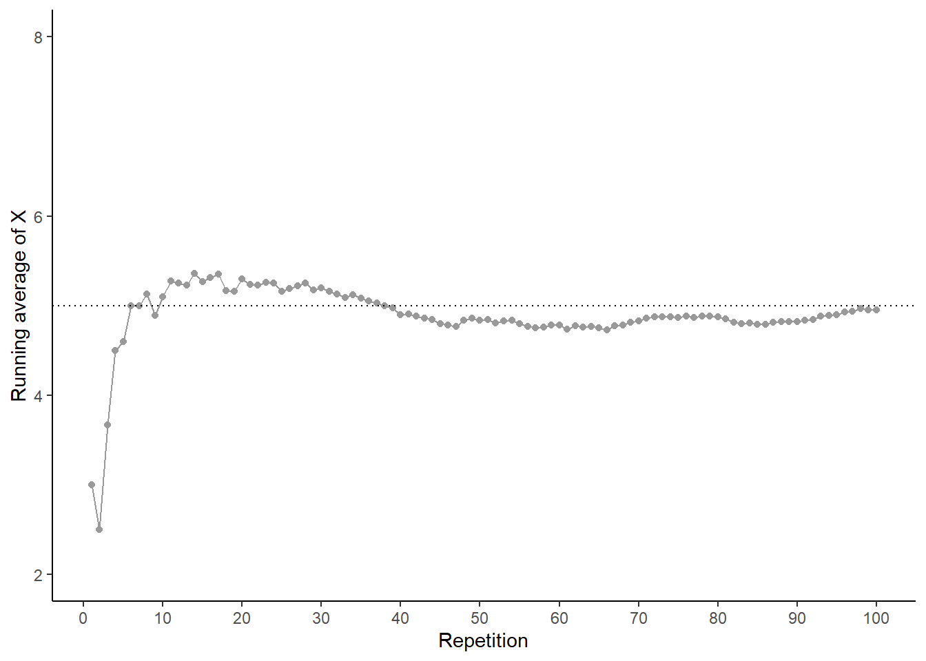
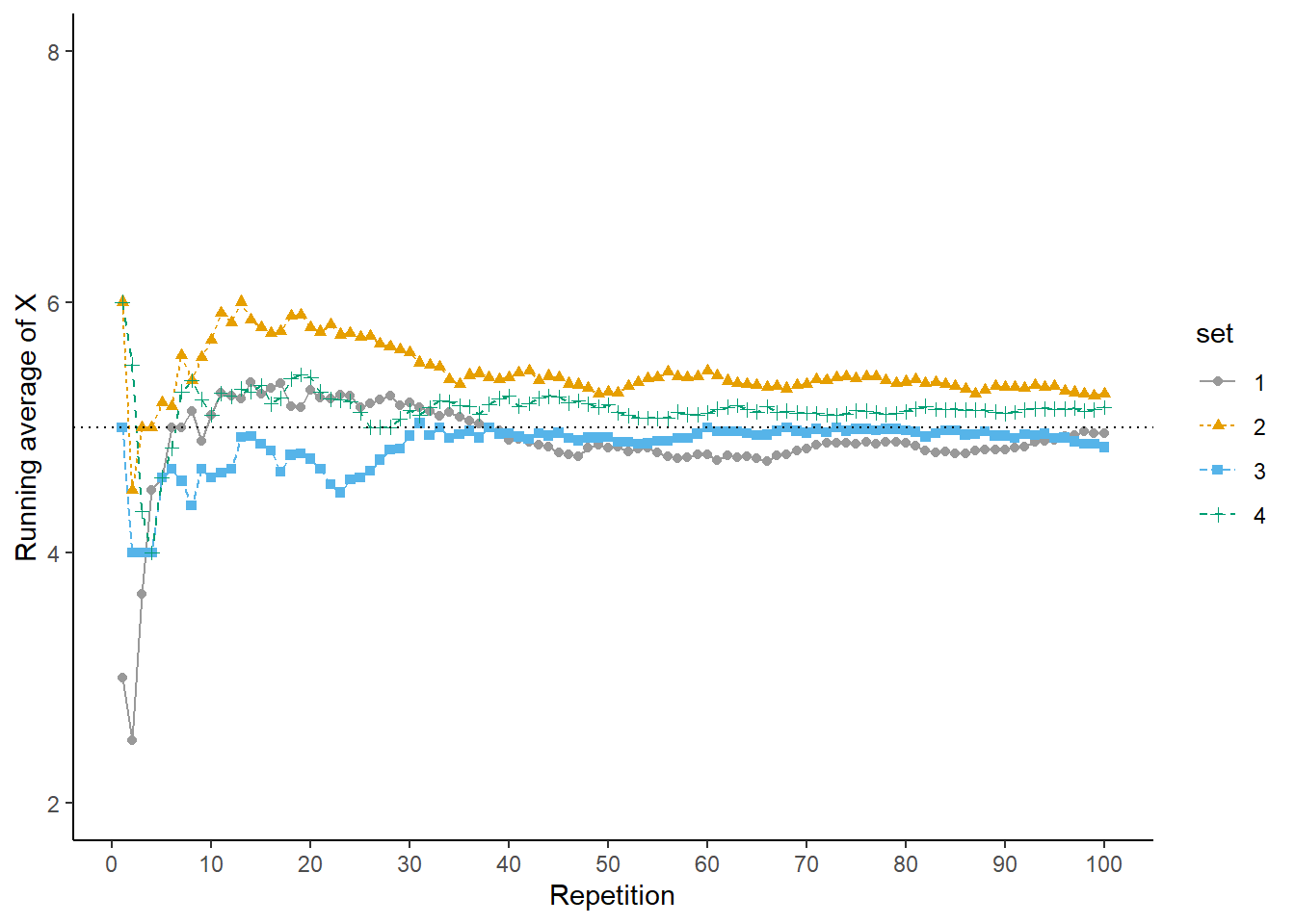
Figure 2.35: Running average of \(X\), the sum of two rolls of a fair four-sided die, for four sets of 100 pairs of rolls.
Now we’ll add 900 more repetitions for a total of 1000 in each set. The plot on the left in Figure 2.36 summarizes the results for our original set, while the plot on the right also displays the results for the three additional sets. Again, the running average of \(X\) fluctuates considerably in the early stages, but settles down and tends to get closer to 5 as the number of repetitions increases. Compared to the results after 100 flips, there is less variability between sets in the running average of \(X\) after 1000 flips: 4.978 (gray), 5.014 (orange), 4.962 (blue), 4.956 (green). Now, even after 1000 repetitions the running average of \(X\) isn’t guaranteed to be exactly 5, but we see a tendency for the running average of \(X\) to get closer to 5 as the number of repetitions increases.
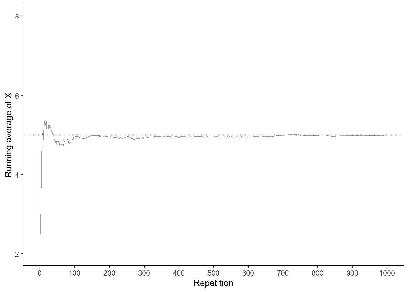

Figure 2.36: Running average of \(X\), the sum of two rolls of a fair four-sided die, for four sets of 1000 pairs of rolls.
Recall the marginal distribution of \(X\), depicted in Figure 2.27. The plot shows that 5 is the “balance point” of the distribution, so we might expect the “true” long run average value of \(X\) to be 5. It is, and our simulation results agree. We will discuss later how to compute the “true” long run average value. For now, we’ll rely on simulation: we can approximate the long run average variable of a random variable \(X\) by simulating many values of \(X\) and finding the average in the usual way.
In Symbulate, we first simulate and store 10000 values of \(X\).
P = BoxModel([1, 2, 3, 4], size = 2)

X = RV(P, sum)

x = X.sim(10000)
We can approximate the long run average value of \(X\) by computing the average — a.k.a., mean — of the 10000 simulated values in the usual way: sum the 10000 simulated values stored in x and divide by 10000. Here are a few ways of computing the mean of the simulated values.
x.sum() / 10000## 4.9814
x.sum() / x.count()## 4.9814
x.mean()## 4.9814Recall that a probability is a theoretical long run relative frequency. A probability can be approximated by a relative frequency from a large number of simulated repetitions, but there is some simulation margin of error.
Likewise, the average value of \(X\) after a large number of simulated repetitions is only an approximation to the theoretical long run average value of \(X\), and there is margin of error due to natural variability in the simulation. The margin of error is also on the order of \(1/\sqrt{N}\) where \(N\) is the number of independently simulated values used to compute the average. However, the degree of variability of the random variable itself also influences the margin of error when approximating long run averages. In particular, if \(\sigma\) is the standard deviation of the random variable, then the margin of error for the average is on the order of \(\sigma / \sqrt{N}\).
Remember that the long run average value is just one feature of a marginal distribution. There is much more to the long run pattern of variability of a random variable that just its average value. We are also interested in percentiles, degree of variability, and quantities that measure relationships between random variables. Two random variables can have the same long run average value but very different distributions. For example, the average temperature in both Phoenix, AZ and Miami, FL is around 75 degrees F, but the distribution of temperatures is not the same.
Next we introduce a few useful properties of averages.
2.9.2 Linearity of averages
Example 2.50 Recall your tactile simulation from Example 2.29. Let \(U_1\) be the result of the first roll, and \(U_2\) the result of the second, so the sum is \(X = U_1 + U_2\).
- Donny Don’t says: “\(X=U_1+U_2\), so I can find the average value of \(X\) by finding the average value of \(U_1\), the average value of \(U_2\), and adding the two averages”. Do you agree? Explain.
- Donny Don’t says: “\(U_1\) and \(U_2\) have the same distribution, so they have the same average value, so I can find the average value of \(X\) by multiplying the average value of \(U_1\) by 2”. Do you agree? Explain.
- Donny Don’t says: “\(U_1\) and \(U_2\) have the same distribution, so \(X=U_1+U_2\) has the same distribution as \(2U_1 = U_1 + U_1\)”. Do you agree? Explain.
Solution. to Example 2.50.
- Donny is correct! Our simulation results are in Table 2.23. The average value of \(U_1\) is \[ \frac{2 + 1 + 3 + 4 + 3 + 3 + 2 + 2 + 1 + 3}{10} = 2.4 \] The average value of \(U_2\) is \[ \frac{1 + 1 + 3 + 3 + 2 + 4 + 3 + 4 + 2 + 4}{10} = 2.7 \] The sum of these two values is equal to the average value of \(X\). To see why, suppose we had just performed two repetitions, resulting in the last two rows of Table 2.23. \[ {\scriptsize \text{Average of $(U_1+U_2)$} = \frac{(1 + 2) + (3 + 4)}{2} = 5 = 2 + 3= \left(\frac{1 + 3}{2}\right)+\left(\frac{2 + 4}{2}\right) = (\text{Average of $U_1$}) + (\text{Average of $U_1$}) } \] We discuss further below.
- Donny is correct that \(U_1\) and \(U_2\) have the same distribution, and he has some good ideas about averages. But we should remind Donny that a distribution represents the long run pattern of variability. With only 10 repetitions, the results for \(U_1\) will not necessarily follow the same pattern as those for \(U_2\). In our simulation, the average value of \(U_1\) is 2.4 and the average value of \(U_2\) is 2.7. Multiplying neither one of these numbers by 2 yields the average value of \(X\). Donny would have been correct if he were talking about long run average values. Since \(U_1\) and \(U_2\) have the same distribution, the long run average value of \(U_1\) is equal to the long run average value of \(U_2\), and so the long run average value of \(X\) is equal to the long run average value of \(U_1\) multiplied by two.
- Donny is not correct. In particular, \(X\) and \(2U_1\) do not have the same possible values; for example, \(X\) can be 3 but \(2U_1\) cannot. The long run average value is just one feature of a distribution. Just because \(X\) and \(2U_1\) have the same long run average value does not necessarily mean they have the same full long run pattern of variability. In particular, relationships between random variables will affect distributions of transformations of them. \(U_1\) and \(U_2\) have the same marginal distribution, but the joint distribution of \((U_1, U_2)\) is not the same as that of \((U_1, U_1)\), and so the distribution of \(U_1+U_2\) is not the same as that of \(U_1+U_1\).
In general the order of transforming and averaging is not interchangeable. However, the order is interchangeable for linear transformations. If \(X\) and \(Y\) are random variables and \(a\) and \(b\) are non-random constants, whether in the short run or the long run, \[ \begin{align*} \text{Average of $a+bX$} & = a+b(\text{Average of $X$})\\ \text{Average of $X+Y$} & = \text{Average of $X$} +\text{Average of $Y$} \end{align*} \] These properties are referred to as linearity of averages. Averaging involves adding and dividing. Linear transformations involve only adding/subtracting and multiplying/dividing. The ability to interchange the order of averaging and linear transformations follows simply from basic properties of arithmetic (commutative, associative, distributive).
Note that the average of the sum of \(X\) and \(Y\) is the sum of the average of \(X\) and the average of \(Y\) regardless of the relationship between \(X\) and \(Y\). We will explore this idea in more detail later.
2.9.3 Averages of indicator random variables
Recall that indicators are the bridge between events and random variables. Indicators are also the bridge between relative frequencies and averages.
Example 2.51 Recall your tactile simulation from Example 2.29. Let \(A\) be the event that the first roll is 3 and \(\textrm{I}_A\) the corresponding indicator random variable. Based only on the results of your simulation, approximate the long run average value of each of \(\textrm{I}_A\). What do you notice?
Solution. to Example 2.51.
Our simulation results are in Table 2.23. Approximate the long run average value of \(\textrm{I}_A\) by summing the 10 simulated values of \(\textrm{I}_A\) and dividing by 10. \[ \frac{0 + 0 + 1 + 0 + 1 + 1 + 0 + 0 + 0 + 1}{10} = \frac{4}{10} \] The average of \(\textrm{I}_A\) is the relative frequency of event \(A\)! When we sum the 1/0 values of \(\textrm{I}_A\) we count the repetitions on which \(A\) occurs. That is, the numerator in the average calculation for \(\textrm{I}_A\) is the frequency of event \(A\), and dividing by the number of repetitions yields the relative frequency of event \(A\).
If \(\textrm{I}_A\) is the indicator random variable of an event \(A\), whether in the short run or the long run, \[ \begin{align*} \text{Average of $\textrm{I}_A$} & = \text{Relative frequency of $A$} \end{align*} \]