2.12 Correlation
Quantities like long run average, variance, and standard deviation summarize characteristics of the marginal distribution of a single random variable. When there are multiple random variables their joint distribution is of interest. Covariance and correlation summarize in a single number a characteristic of the joint distribution of two random variables, namely, the degree to which they “co-deviate from the their respective means”.
Covariance is the average of the paired deviations from the respective means. Let \(T\) and \(W\) be the first arrival time and waiting time random variables from the meeting problem in the previous section. Recall that we have already simulated some \((T, W)\) pairs
t_and_w| Index | Result |
|---|---|
| 0 | (19.66959340251227, 18.730712326991387) |
| 1 | (29.201822361960236, 4.76153849445895) |
| 2 | (36.16481074855953, 13.026780147992625) |
| 3 | (31.039382871024436, 13.692197808075413) |
| 4 | (27.11888898469543, 9.940077174498654) |
| 5 | (17.50009085957651, 18.443124984246253) |
| 6 | (16.003805989072546, 14.741604171385937) |
| 7 | (18.18570029790294, 15.461451185395767) |
| 8 | (15.323787134263348, 10.913167237349086) |
| ... | ... |
| 9999 | (25.249121207913834, 20.345080862179994) |
The simulated long run averages are (notice that calling mean returns the pair of averages)
t_and_w.mean()## (24.38056155450146, 11.275765734293687)Now within each simulated \((t, w)\) pair, we subtract the mean of the \(T\) values from \(t\) and the mean of the \(W\) values from \(w\),
We can do this subtract in a “vectorized” way: the following code subtracts the first component of t_and_w.mean() (the average of the \(T\)) from the first component of each of the t_and_w values (the individual \(t\) value), and similarly for the second.
t_and_w - t_and_w.mean()| Index | Result |
|---|---|
| 0 | (-4.710968151989189, 7.4549465926977) |
| 1 | (4.821260807458778, -6.514227239834737) |
| 2 | (11.784249194058074, 1.7510144136989378) |
| 3 | (6.658821316522978, 2.416432073781726) |
| 4 | (2.738327430193973, -1.3356885597950328) |
| 5 | (-6.880470694924949, 7.1673592499525665) |
| 6 | (-8.376755565428912, 3.46583843709225) |
| 7 | (-6.194861256598518, 4.18568545110208) |
| 8 | (-9.05677442023811, -0.3625984969446012) |
| ... | ... |
| 9999 | (0.8685596534123761, 9.069315127886307) |
For each simulated pair, we now have a pair of deviations from the respective mean. To measure the interaction between these deviations, we take the product of the deviations within each pair. First, we split the paired deviations into two separate columns and then take the product within each row
t_deviations = (t_and_w - t_and_w.mean())[0] # first column (Python 0)
w_deviations = (t_and_w - t_and_w.mean())[1] # second column (Python 1)

t_deviations * w_deviations| Index | Result |
|---|---|
| 0 | -35.12001597297918 |
| 1 | -31.40678848229559 |
| 2 | 20.63439019341578 |
| 3 | 16.090589402827582 |
| 4 | -3.6575526214830205 |
| 5 | -49.31480527929789 |
| 6 | -29.03248141678995 |
| 7 | -25.929740633340362 |
| 8 | 3.2839727919446506 |
| ... | ... |
| 9999 | 7.87724120416455 |
Now we take the average of the products of the paired deviations.
(t_deviations * w_deviations).mean()## -36.82999736207149This value is the covariance, which we could have arrived at more quickly by calling cov on the simulated pairs.
t_and_w.cov()## -36.829997362071495The covariance of random variables \(X\) and \(Y\) is defined as the long run average of the product of the paired deviations from the respective means
\[ \text{Covariance($X$, $Y$)} = \text{Average of} ((X - \text{Average of }X)(Y - \text{Average of }Y)) \] It turns out that covariance is equivalent to the average of the product minus the product of the averages.
\[ \text{Covariance($X$, $Y$)} = \text{Average of} XY - (\text{Average of }X)(\text{Average of }Y) \]
(t_and_w[0] * t_and_w[1]).mean() - (t_and_w[0].mean()) * (t_and_w[1].mean()) ## -36.82999736207151Unfortunately, the value of covariance is hard to interpret as it depends heavily on the measurement unit scale of the random variables. In the meeting problem, covariance is measured in squared-minutes. If we converted the \(T\) values from minutes to seconds, then the value of covariance would change accordingly and would be measured in (minutes \(\times\) seconds).
But the sign of the covariance does have practical meaning.
- A positive covariance indicate an overall positive association: above average values of \(X\) tend to be associated with above average values of \(Y\)
- A negative covariance indicates am overall negative association: above average values of \(X\) tend to be associated with below average values of \(Y\)
- A covariance of zero indicates that the random variables are uncorrelated: there is no overall positive or negative association. But be careful: if \(X\) and \(Y\) are uncorrelated there can still be a relationship between \(X\) and \(Y\). We will see examples later that demonstrate that being uncorrelated does not necessarily imply that random variables are independent.
Example 2.57 Consider the probability space corresponding to two rolls of a fair four-sided die. Let \(X\) be the sum of the two rolls, \(Y\) the larger of the two rolls, \(W\) the number of rolls equal to 4, and \(Z\) the number of rolls equal to 1. Without doing any calculations, determine if the covariance between each of the following pairs of variables is positive, negative, or zero. Explain your reasoning conceptually.
- \(X\) and \(Y\)
- \(X\) and \(W\)
- \(X\) and \(Z\)
- \(X\) and \(V\), where \(V = W + Z\).
- \(W\) and \(Z\)
Solution. to Example 2.57
Show/hide solution
- Positive. There is an overall positive association; above average values of \(X\) tend to be associated with above average values of \(Y\) (e.g., (7, 4), (8, 4)), and below average values of \(X\) tend to be associated with below average values of \(Y\) (e.g., (2, 1), (3, 2)).
- Positive. If \(W\) is large (roll many 4s) then \(X\) (sum) tends to be large.
- Negative. If \(Z\) is large (roll many 1s) then \(X\) (sum) tends to be small.
- Zero.. Basically, the positive association between \(X\) and \(W\) cancels out with the negative association of \(X\) and \(Z\). \(V\) is large when there are many 1s or many 4s, or some mixture of 1s and 4s. So knowing that W is large doesn’t really tell you anything about the sum.
- Negative. There is a fixed number of rolls. If you roll lots of 4s (\(W\) is large) then there must be few rolls of 1s (\(Z\) is small).
The numerical value of the covariance depends on the measurement units of both variables, so interpreting it can be difficult. Covariance is a measure of joint association between two random variables that has many nice theoretical properties, but the correlation (coefficient) is often a more practical measure. (We saw a similar idea with variance and standard deviation. Variance has many nice theoretical properties. However, standard deviation is often a better practical measure of variability.)
The correlation for two random variables is the covariance between the corresponding standardized random variables. Therefore, correlation is a standardized measure of the association between two random variables.
Returning to the \((T, W)\) example, we carry out the same process, but first standardize each of the simulated values of \(T\) by subtracting their mean and dividing by their standardization, and similarly for \(W\).
t_and_w.standardize()| Index | Result |
|---|---|
| 0 | (-0.5719496146421935, 0.8788285426420563) |
| 1 | (0.5853400345640645, -0.7679315687158395) |
| 2 | (1.4307031098359593, 0.2064188423353166) |
| 3 | (0.8084347342378895, 0.28486179631055475) |
| 4 | (0.3324550852253745, -0.15745803351269363) |
| 5 | (-0.8353447604729765, 0.8449262252794381) |
| 6 | (-1.017005838932683, 0.4085713700063412) |
| 7 | (-0.7521062325537683, 0.49343074416566285) |
| 8 | (-1.09956562482156, -0.042745029045031795) |
| ... | ... |
| 9999 | (0.10545016290403181, 1.0691388459320488) |
Now we compute the covariance of the standardized values.
t_and_w.standardize().cov()## -0.5271192883725944Recall that we already computed the correlation in the previous section.
t_and_w.standardize().corr()## -0.5271192883725928We see that the correlation is the covariance of the standardized random variables.
\[ \text{Correlation}(X, Y) = \text{Covariance}\left(\frac{X- \text{Average of }X}{\text{Standard Deviation of }X}, \frac{Y- \text{Average of }Y}{\text{Standard Deviation of }Y}\right) \]
When standardizing, subtracting the means doesn’t change the scale of the possible pairs of values; it merely shifts the center of the joint distribution. Therefore, correlation is the covariance divided by the product of the standard deviations.
\[ \text{Correlation}(X, Y) = \frac{\text{Covariance}(X, Y)}{(\text{Standard Deviation of }X)(\text{Standard Deviation of }Y)} \]
A correlation coefficient has no units and is measured on a universal scale. Regardless of the original measurement units of the random variables \(X\) and \(Y\) \[ -1\le \textrm{Correlation}(X,Y)\le 1 \]
- \(\textrm{Correlation}(X,Y) = 1\) if and only if \(Y=aX+b\) for some \(a>0\)
- \(\textrm{Correlation}(X,Y) = -1\) if and only if \(Y=aX+b\) for some \(a<0\)
Therefore, correlation is a standardized measure of the strength of the linear association between two random variables. The closer the correlation is to 1 or \(-1\), the closer the joint distribution of \((X, Y)\) pairs hugs a straight line, with positive or negative slope.
Because correlation is computed between standardized random variables, correlation is not affected by a linear rescaling of either variable. One standard deviation above the mean is one standard deviation above the mean, whether that’s measured in feet or inches or meters.
2.12.1 Joint Normal distributions
Just as Normal distributions are commonly assumed for marginal distributions of individual random variables, joint Normal distributions are often assumed for joint distributions of several random variables. We’ll focus “Bivariate Normal” distributions which describe a specific pattern of joint variability for two random variables.
Example 2.58 Donny Don’t has just completed a problem where it was assumed that SAT Math scores follow a Normal(500, 100) distribution. Now a follow up problem asks Donny how he could simulate a single (Math, Reading) pair of scores. Donny says: “That’s easy; just spin the Normal(500, 100) twice, once for Math and once for Reading.” Do you agree? Explain your reasoning.
Solution. to Example 2.58
Show/hide solution
You should not agree with Donny, for two reasons.
- It’s possible that the distribution of SAT Math scores follow a different pattern than SAT Reading scores. So we might need one spinner to simulate a Math score, and a second spinner to simulate the Reading score. (In reality, SAT Math and Reading scores do follow pretty similar distributions. But it’s possible that they could follow different distributions.)
- Furthermore, there is probably some relationship between scores. It is plausible that students who do well on one test tend to do well on the other. For example, students who score over 700 on Math are probably more likely to score above than below average on Reading. If we simulate a pair of scores by spinning one spinner for Math and a separate spinner for Reading, then there will be no relationship between the scores because the spins are physically independent.
In the previous problem, hat we really need is a spinner that generates a pair of scores simultaneously to reflect their association. This is a little harder to visualize, but we could imagine spinning a “globe” with lines of latitude corresponding to SAT Math score and lines of longitutde to SAT Reading score. But this would not be a typical globe:
- The lines of latitude would not be equally spaced, since SAT Math scores are not equally likely. (We have seen similar issues for one-dimensional Normal spinners.) Similarly for lines of longitude.
- The scale of the lines of latitude would not necessarily match the scale of the lines of longitude, since Math and Reading scores could follow difference distributions. For example, the equator (average Math) might be 500 while the prime meridian (average Reading) might be 520.
- The “lines” would be tilted or squiggled to reflect the relationship between the scores. For example, the region corresponding to Math scores near 700 and Reading scores near 700 would be larger than the region corresponding to Math scores near 700 but Reading scores near 200.
So we would like a model that
- Simulates Math scores that follow a Normal distribution pattern, with some mean and some standard deviation.
- Simulates Reading scores that follow a Normal distribution pattern, with possibly a different mean and standard deviation.
- Reflects how strongly the scores are associated.
Such a model is called a “Bivariate Normal” distribution. There are five parameters: the two means, the two standard deviations, and the correlation which reflects the strength of the association between the two scores.
We have already encountered a Bivariate Normal model. Recall that in one case of the meeting problem we assumes that Regina and Cady tend to arrive around the same time. One way to model pairs of values that have correlation is with a BivariateNormal distribution, like in the following. We assumed a Bivariate Normal distribution for the \((R, Y)\) pairs, with mean (30, 30), standard deviation (10, 10) and correlation 0.7. (We could have assumed different means and standard deviations.)
R, Y = RV(BivariateNormal(mean1 = 30, sd1 = 10, mean2 = 30, sd2 = 10, corr = 0.7))

(R & Y).sim(1000).plot()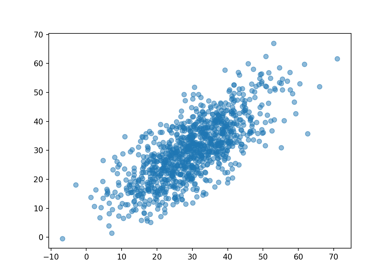
Now we see that the points tend to follow the \(R = Y\) line, so that Regina and Cady tend to arrive near the same time, similar to Figure 2.11.
Recall that in some of the previous examples the shapes of one-dimensional histograms could be approximated with a smooth density curve. Similarly, a two-dimensional histogram can sometimes be approximated with a smooth density surface. As with histograms, the height of the density surface at a particular \((X, Y)\) pair of values can be represented by color intensity. A marginal Normal distribution is a “bell-shaped curve”; a Bivariate Normal distribution is a “mound-shaped” curve — imagine a pile of sand. (Symbulate does not yet have the capability to display densities in a three-dimensional-like plot such as this plot.)
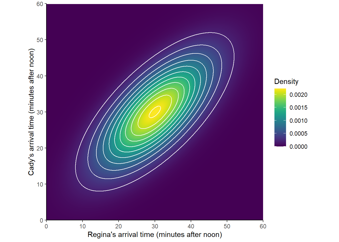
Figure 2.41: A Bivariate Normal distribution