2.4 Probability spaces

In the previous sections in the chapter we defined outcomes, events, and random variables, the main mathematical objects associated with a random phenomenon. But we haven’t actually computed any probabilities yet! So far we have only been concerned with what is possible. You might have noticed that the examples often did not include any assumptions like the “die is fair”, “each object is equally likely to be put in any spot”, or “Regina is more likely to arrive late and Cady is more likely to arrive early”. Now we will start to incorporate assumptions of the random phenomenon to determine how probable various events are.

A probability measure, typically denoted $\textrm{P}$, assigns probabilities to events to quantify their relative likelihoods according to the assumptions of the model of the random phenomenon. The probability of event $A$ is denoted $\textrm{P}(A)$. An event is something that can happen; $\textrm{P}(A)$ quantifies how likely it is that $A$ will happen.

As we saw in Section 1.3, there are some basic logical consistency requirements that probabilities must satisfy. A valid probability measure $\textrm{P}$ must satisfy the following three “axioms”.

For any event $A$, $0 \le \textrm{P}(A) \le 1$.
If $\Omega$ represents²⁶ the sample space then $\textrm{P}(\Omega) = 1$.
(Countable additivity.) If $A_1, A_2, A_3, \ldots$ are disjoint²⁷ events, then \[ \textrm{P}(A_1 \cup A_2 \cup A_2 \cup \cdots) = \textrm{P}(A_1) + \textrm{P}(A_2) +\textrm{P}(A_3) + \cdots \]

The above axioms require that probabilities of different events must fit together in a valid, logically coherent way.

The requirement $0\le \textrm{P}(A)\le 1$ makes sense in light of the relative frequency interpretation: an event $A$ can not occur on more than 100% of repetitions or less than 0% of repetitions of the random phenomenon.

The requirement that $\textrm{P}(\Omega)=1$ just ensures that the sample space accounts for all of the possible outcomes. Basically, $\textrm{P}(\Omega)=1$ says that on any repetition of the random phenomenon, “something has to happen”. Roughly, $\textrm{P}(\Omega)=1$ implies that all outcomes taken together need to account for 100% of the probability. If $\textrm{P}(\Omega)$ were less than 1, then the sample space hasn’t accounted for all of the possible outcomes.

Countable addivity says that as long as events share no outcomes in common, then the probability that at least one of the events occurs is equal to the sum of the probabilities of the individual events. In Example 1.4, the events $A$=“the Astros win the 2022 World Series” and $D$=“the Dodgers win the 2022 World Series” are disjoint, $A\cap D = \emptyset$; in a single World Series, both teams cannot win. If $\textrm{P}(A) = 0.2$ and $\textrm{P}(B) = 0.09$, then the probability of $A\cup D$, the event that either the Astros or the Dodgers win, must be $\textrm{P}(A\cup D)=0.29$.

Countable additivity can be understood through a diagram with areas representing probabilities, as in the figure below which represents two events (yellow / and blue \). On the left, there is no “overlap” between areas so the total area is the sum of the two pieces; this depicts countable additivity for two disjoint events. On the right, there is overlap between the two areas, so simply adding the two areas “double counts” the intersection (green $\times$) and does not result in the correct total area. Countable additivity applies to any countable number²⁸ of events, as long as there is no “overlap”.

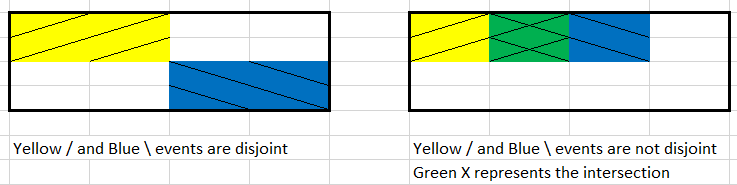
Figure 2.5: Illustration of countable additivity for two events. The events in the picture on the left are disjoint, but not on the right.

Many other properties follow from the axioms, some of which we have already used intuitively when constructing two-way tables.

Complement rule²⁹. For any event $A$, $\textrm{P}(A^c) = 1 - \textrm{P}(A)$.
Subset rule³⁰. If $A \subseteq B$ then $\textrm{P}(A) \le \textrm{P}(B)$.
Addition rule for two events³¹. If $A$ and $B$ are any two events \[\begin{align*} \textrm{P}(A\cup B) = \textrm{P}(A) + \textrm{P}(B) - \textrm{P}(A \cap B) \end{align*}\]
Law of total probability. If $C_1, C_2, C_3\ldots$ are disjoint events with $C_1\cup C_2 \cup C_3\cup \cdots =\Omega$, then \[\begin{align*} \textrm{P}(A) & = \textrm{P}(A \cap C_1) + \textrm{P}(A \cap C_2) + \textrm{P}(A \cap C_3) + \cdots \end{align*}\]

The main “meat” of the axioms is countable additivity. Thus, the key to many proofs of probability properties is to write relevant events in terms of disjoint events.

Example 2.17 Donny Don’t says: “Wait a minute. You said unions are inclusive; $\textrm{P}(A\cup B)$ means the probability of $A$ or $B$ OR BOTH. So $\textrm{P}(A\cup B)$ should just be $\textrm{P}(A)+\textrm{P}(B)$.” Explain to Donny his mistake, using the picture on the right in Figure 2.5 as an example.

Solution. to Example 2.17.

Show/hide solution

$A\cup B$ is inclusive so we do want to count the possibility of both, $A\cap B$. The problem with simply adding $\textrm{P}(A)$ and $\textrm{P}(B)$ is that their sum double counts $A \cap B$. We do want to count the outcomes that satisfy both $A$ and $B$, but we only want to count them once. Subtracting $\textrm{P}(A \cap B)$ in the general addition rule for two events corrects for the double counting.

For example, consider the picture on the right in Figure 2.5. Suppose each rectangular cell represents a distinct outcome; there are 16 outcomes in total. Assume the outcomes are equally likely, each with probability $1/16$. Let $A$ represent the yellow / event which has probability $4/16$ and let $B$ represent the blue \ event which has probability 4/16. (Remember, green represents outcomes that satisfy both blue and yellow.) Then $\textrm{P}(A\cup B) = 6/16$, since there are 6 outcomes which satisfy either event $A$ or $B$ (or both). However, simply adding $\textrm{P}(A)+\textrm{P}(B)$ yields $8/16$ because the two outcomes that satisfy the green event $A\cap B$ are counted both in $\textrm{P}(A)$ and $\textrm{P}(B)$. So to correct for this double counting, we subtract out $\textrm{P}(A\cap B)$: \[ \textrm{P}(A)+\textrm{P}(B)-\textrm{P}(A\cap B) = 4/16 + 4/16 -2/16 = 6/16 = \textrm{P}(A\cup B) \]

Warning: The general addition rule for more than two events is more complicated³²; see the inclusion-exclusion principle.

The complement rule follows from the fact that an event either happens or it doesn’t. We’ll see that it is sometimes more convenient to compute directly the probability that an event does not happen and then use the complement rule. Subtracting a computed probability from 1 seems like a small computational step, but it’s an important one. A basketball player who has a 90% chance of successfully making a free throw is much different from a player who only has a 10% chance. Unfortunately, the complement rule step is often overlooked when doing probability calculations. It’s a good idea to ask yourself if the probability you are computing should be greater than or less than 50%. If your computed value seems to be on the wrong side of 50%, check your calculations to see if you have forgotten (or misapplied) the complement rule.

The complement rule is often useful in probability problems that involve finding “the probability of at least one…,” which on the surface involves unions (OR). However, the general addition rule for multiple events is complicated and not very useful. Therefore, it usually more convenient to use the complement rule and compute “the probability of at least one…” as one minus “the probability of none…”; the latter probability involves intersections (AND). We will see more about probabilities of intersections later.

In the law of total probability the events $C_1, C_2, C_3, \ldots$, which represent “cases”, form a partition of the sample space; each outcome in the sample space satisfies exactly one of the cases $C_i$. The law of total probability says that we can compute the “overall” probability $\textrm{P}(A)$ by summing the probabilities of $A$ in each “case” $\textrm{P}(A\cap C_i)$. The law of total probability basically says that we can sum across rows and columns in two-way tables. (Later we will see a different and more useful expression of the law of total probability, involving conditional probabilities.)

The following example is one we have basically covered before, but now we introduce some more mathematical notation. The example involves randomly selecting a U.S. household. Note that while “randomly select” is commonly used terminology, it is not the best wording. Remember that “random” simply means uncertain, so technically “randomly select” just means selecting in a way that the outcome is uncertain. Suppose I want to “randomly select” one of two households, A or B. I could put 10 tickets in a hat, with 9 labeled A and 1 labeled B, and then draw a ticket; this is random selection because the outcome of the draw is uncertain. However, what is often meant by “randomly select” is selecting in a way that each outcome is equally likely. To give households A and B the same chance of being selected, I would put a single ticket for each in the hat. Randomly selecting in a way that each outcome is equally likely could be described more precisely as “selecting uniformly at random”. (We will discuss equally likely outcomes in more detail later.)

Example 2.18 The probability that a randomly selected U.S. household has a pet dog is 0.47. The probability that a randomly selected U.S. household has a pet cat is 0.25. (These values are based on the 2018 General Social Survey (GSS).)

Represent the information provided using proper symbols.
Donny Don’t says: “the probability that a randomly selected U.S. household has a pet dog OR a pet cat is $0.47 + 0.25=0.72$.” Do you agree? What must be true for Donny to be correct? Explain.
What is the largest possible value of the probability that a randomly selected U.S. household has a pet dog AND a pet cat? Describe the (unrealistic) situation in which this extreme case would occur. (Hint: for the remaining parts it helps to consider two-way tables.)
What is the smallest possible value of the probability that a randomly selected U.S. household has a pet dog AND a pet cat? Describe the (unrealistic) situation in which this extreme case would occur.
Donny Don’t says: “I remember hearing once that in probability OR means add and AND means multiply. So the probability that a randomly selected U.S. household has a pet dog AND a pet cat is $0.47 \times 0.25=0.1175$.” Do you agree? Explain.
According to the GSS, the probability that a randomly selected U.S. household has a pet dog AND a pet cat is $0.15$. Compute the probability that a randomly selected U.S. household has a pet dog OR a pet cat.
Compute and interpret $\textrm{P}(C \cap D^c)$.

Solution. to Example 2.18.

Show/hide solution

This is basically just Example 1.11 again. Here we introduce more mathematical notation, but the ideas are the same as we discussed in Example 1.11.

The sample space consists of U.S. households. Let $C$ be the event that the household has a pet cat, and let $D$ be the event that the household has a pet dog. Let $\textrm{P}$ be the probability measure corresponding to randomly selecting a U.S. household. (The probability measure corresponds to however the random selection is done; though not specified, it’s assumed to be uniformly at random.) Then $\textrm{P}(C) = 0.25$ and $\textrm{P}(D) = 0.47$.
Donny would be correct if the events $C$ and $D$ were disjoint, which would only be true if the probability that a randomly selected U.S. household has a pet dog AND a pet cat were 0. This is unrealistic, since I’m sure you know households (maybe even your own!) that have both pet cats and dogs.
$\textrm{P}(C \cup D) = \textrm{P}(C) + \textrm{P}(D) - \textrm{P}(C \cap D) = 0.25 + 0.42 - \textrm{P}(C\cap D)$. So $\textrm{P}(C\cup D)$ is the largest it can be when $\textrm{P}(C \cap D)$ is the smallest it can be. The smallest $\textrm{P}(C \cap D)$ can be is 0, and hence the largest $\textrm{P}(C\cup D)$ can be is 0.72, which would only be true if no households had both a pet cat and a pet dog. The following two-way table of percents represents this unrealistic scenario.

D not D Total

C 0 25 25

not C 47 28 75

Total 47 53 100
$\textrm{P}(C \cup D) = \textrm{P}(C) + \textrm{P}(D) - \textrm{P}(C \cap D) = 0.25 + 0.42 - \textrm{P}(C\cap D)$. $\textrm{P}(C\cup D)$ is the smallest it can be when $\textrm{P}(C \cap D)$ is the largest it can be. The probability that the household has both a pet cat and a pet dog can not be larger than either of the two component probabilities; that is $\textrm{P}(C\cap D)\le \textrm{P}(C) = 0.25$ and $\textrm{P}(C\cap D)\le \textrm{P}(D) = 0.42$. The largest $\textrm{P}(C \cap D)$ can be is 0.25, and hence the smallest $\textrm{P}(C\cup D)$ can be is 0.42, which would only be true if every household that has a pet cat also has a pet dog. The following two-way table of percents represents this unrealistic scenario.

D not D Total

C 25 0 25

not C 22 53 75

Total 47 53 100
Tell Donny to check the axioms of probability. There is no requirement that the probability of an intersection must be the product of the probabilities. The two previous parts show that $0\le \textrm{P}(C \cap D) \le 0.25$, but without further information we can’t determine the value of $\textrm{P}(C\cap D)$. It helps to think it in percentage terms. The extreme of 0 occurs when 0% of households with a pet cat also have a pet dog; the extreme of 0.25 occurs when 100% of households with a pet cat also have a pet dog. We might expect that that the true value of $\textrm{P}(C \cap D)$ depends on the actual percentage of households with a pet cat that also have a pet dog. Without knowing that percentage (or equivalent information), we cannot determine $\textrm{P}(C \cap D)$. (We will explore this topic in more depth later.)
$\textrm{P}(C \cup D) = \textrm{P}(C) + \textrm{P}(D) - \textrm{P}(C \cap D) = 0.25 + 0.42 - 0.15 = 0.52$. Notice that this is between the hypothetical extremes of 0.42 and 0.72. Also notice that the actual $\textrm{P}(C \cap D)$ is between the hypothetical extremes of 0 and 0.25, but it is not equal to the product of 0.25 and 0.42. The moral is that we are not able to compute probabilities involving both events ($\textrm{P}(C\cup D)$, $\textrm{P}(C \cap D$)) based on the probability of each event alone. The following two-way table of percents represents the actual scenario.

D not D Total

C 15 10 25

not C 32 43 75

Total 47 53 100
The law of total probability implies that $\textrm{P}(C) = \textrm{P}(C \cap D) + \textrm{P}(C \cap D^c)$ so $\textrm{P}(C \cap D^c) = 0.11$. An adult either has a dog or not (the two cases); if 14% of adults have both a cat and a dog and 11% of adults have a cat but no dog, then 25% of adults have a cat.

	D	not D	Total
C	0	25	25
not C	47	28	75
Total	47	53	100

	D	not D	Total
C	25	0	25
not C	22	53	75
Total	47	53	100

	D	not D	Total
C	15	10	25
not C	32	43	75
Total	47	53	100

Probabilities involving multiple events, such as $\textrm{P}(A \cap B)$ or $\textrm{P}(X>80, Y<2)$, are often called joint probabilities. Note that the axioms do not specify any direct requirements on probabilities of intersections. In particular, is not necessarily true that $\textrm{P}(A\cap B)$ equals $\textrm{P}(A)\textrm{P}(B)$. It is true that probabilities of intersections can be obtained by multiplying, but the product generally involves at least one conditional probability that reflects any association between the events involved. In general, joint probabilities ($\textrm{P}(A \cap B)$) can not be computed based on the individual probabilities ($\textrm{P}(A)$, $\textrm{P}(B)$) alone. We will explore this topic in more depth later.

Example 2.19 Consider a Cal Poly student who frequently has blurry, bloodshot eyes, generally exhibits slow reaction time, always seems to have the munchies, and disappears at 4:20 each day. Which of the following events, $A$ or $B$, has a higher probability? (Assume the two probabilities are not equal.)

$A$: The student has a GPA above 3.0.
$B$: The student has a GPA above 3.0 and smokes marijuana regularly.

Solution. to Example 2.19.

Show/hide solution

$A$ has the higher probability. Many people say $B$, associating the description of the student with the “smokes marijuana regularly” part of event $B$. But every student who satisfies event $B$ also satisfies event $A$, so $\textrm{P}(A)$ can’t be any smaller than $\textrm{P}(B)$. That is, $B\subseteq A$ so $\textrm{P}(B) \le \textrm{P}(A)$.

Warning! Your psychological judgment of probabilities is often inconsistent with the mathematical logic of probabilities.

Probabilities are always defined for events (sets) but remember than many events are defined in terms of random variables. For example, if $X$ is tomorrow’s high temperature (degrees F) we might be interested in $\textrm{P}(\{X>80\})$, the probability of the event that tomorrow’s high temperature is above 80 degrees F. If $Y$ is the amount of rainfall tomorrow (inches) we might be interested in $\textrm{P}(\{X > 80\}\cap \{Y < 2\})$, the probability of the event that tomorrow’s high temperature is above 80 degrees F and the amount of rainfall is less than 2 inches. To simplify notation, it is common to write $\textrm{P}(X>80)$ instead of $\textrm{P}(\{X>80\})$, or $\textrm{P}(X > 80, Y < 2)$ instead of $\textrm{P}(\{X > 80\}\cap \{Y < 2\})$. Read the comma in $\textrm{P}(X > 80, Y < 2)$ as “and”. But keep in mind that an expression like “$X>80$” really represents an event $\{X>80\}$.

A probability model (or probability space) puts all the objects we have seen so far in this chapter together in a model for the random phenomenon. Think of a probability space as the collection of all outcomes, events, and random variables associated with a random phenomenon along with the probabilities of all events of interest under the assumptions of the model.

Before we work with some numerical probabilities, let’s pause briefly to think about some of the concepts we have seen so far. It’s easy to get confused between things like events, random variables, and probabilities, and the symbols that represent them. But a strong understanding of these fundamental concepts will help you solve probability problems. Examples like the following do more than encourage proper use of notation. Explaining to Donny why he is wrong will help you better understand the objects that symbols represent, how they are different from one another, and how they connect to real-world contexts.

Example 2.20 (Don’t do what Donny Don’t does.) At various points in his homework, Donny Don’t writes the following. Explain to Donny why each of the following symbols is nonsense, both mathematically and intuitively using a simple example (like tomorrow’s weather). Below, $A$ and $B$ represent events, $X$ and $Y$ represent random variables.

$\textrm{P}(A = 0.5)$
$\textrm{P}(A + B)$
$\textrm{P}(A) \cup \textrm{P}(B)$
$\textrm{P}(X)$
$\textrm{P}(X = A)$
$\textrm{P}(X \cap Y)$

Solution. to Example 2.20

Show/hide solution

We’ll respond to Donny using tomorrow’s weather as an example, with $A$ representing the event that it rains tomorrow, $X$ tomorrow’s high temperature (degrees F), $B=\{X>80\}$ the event that tomorrow’s high temperature is above 80 degrees, and $Y$ tomorrow’s rainfall (inches).

$A$ is a set and 0.5 is a number; it doesn’t make mathematical sense to equate them. It doesn’t make sense to say “it rains tomorrow equals 0.5”. Donny probably means “the probability that it rains tomorrow equals 0.5” which he should write as $\textrm{P}(A) = 0.5$.
$A$ and $B$ are sets; it doesn’t make mathematical sense to add them. The symbol $A + B$ would represent “it rains tomorrow plus tomorrow’s high temperature is above 80 degrees F,” where “plus” literally means the mathematical sum. Donny might mean “the probability that (it rains tomorrow) or (tomorrow’s high temperature is above 80 degrees),” which he should write as $\textrm{P}(A \cup B)$. Donny might have meant to write $\textrm{P}(A) + \textrm{P}(B)$, which is valid expression since $\textrm{P}(A)$ and $\textrm{P}(B)$ are numbers. However, he should keep in mind that $\textrm{P}(A) + \textrm{P}(B)$ is not necessarily a probability of anything; this sum could even be greater than one. In particular, since there are some rainy days with high temperatures above 80 degrees — that is, $A$ and $B$ are not disjoint — $\textrm{P}(A) + \textrm{P}(B)$ is greater than $\textrm{P}(A\cup B)$. (See the general addition rule and related discussion in Section ??.) Donny might also mean “the probability that (it rains tomorrow) and (tomorrow’s high temperature is above 80 degrees),” which he should write as $\textrm{P}(A \cap B)$.
$\textrm{P}(A)$ and $\textrm{P}(B)$ are numbers; union is an operation on sets, and it doesn’t make mathematical sense to take a union of numbers. See the previous part for related discussion.
$X$ is a random variable, and probabilities are assigned to events. $P(X)$ reads “the probability that tomorrow’s high temperature in degrees F”, a subject in need of a predicate; the phrase is missing any qualifying information that could define an event. We assign probabilities to things that might happen (events) like “tomorrow’s high temperature is above 80 degrees,” which has probability $\textrm{P}(X > 80)$.
$X$ is a random variable (a function) and $A$ is an event (a set), and it doesn’t make sense to equate these two different mathematical objects. It doesn’t make sense to say “tomorrow’s high temperature in degrees F equals the event that it rains tomorrow”. We’re not sure what Donny was thinking here.
$X$ and $Y$ are RVs (functions) and intersection is an operation on sets. $X \cap Y$ is attempting to say “tomorrow’s high temperature in degrees F and the amount of rainfall in inches tomorrow”, but this is still missing qualifying information to define a valid event for which a probability can be assigned. We could say $\textrm{P}(X > 80, Y < 2)$ to represent “the probability that (tomorrow’s high temperature is greater than 80 degrees F) AND (the amount of rainfall tomorrow is less than 2 inches)”. (Remember,“$X > 80, Y < 2$” is short for the event $\{X > 80\} \cap \{Y < 2\}$.) If we want to say something like “we measure tomorrow’s high temperature in degrees F and the amount of rainfall in inches tomorrow” we would write $(X, Y)$.

2.4.1 Some probability measures for a four-sided die

The three axioms (and related properties) of a probability measure are simply minimal logical consistency requirements that must be satisfied by any probability model to ensure that probabilities fit together in a coherent way. There are also many physical aspects of the random phenomenon or assumptions (e.g. “fairness”, independence, conditional relationships) that must be considered when determining a reasonable probability measure for a particular situation. Sometimes $\textrm{P}(A)$ is defined explicitly for an event $A$ via a formula. But it is much more common for a probability measure to be defined only implicitly through modeling assumptions; probabilities of events then follow from the axioms and related properties.

Consider a single roll of a four-sided die. Careful: other examples in this chapter have involved a pair of rolls, but here we are just considering one roll. The sample space consists of four possible outcomes $\Omega = \{1, 2, 3, 4\}$. Events concern what might happen on a single roll. For example, if $A$ is the event that we roll an odd number then $A = \{1, 3\}$, consisting of the outcomes 1 and 3.

Let’s first assume that the die is fair, so all four outcomes are equally likely, each with probability³³ 1/4. Given that the probability of each outcome³⁴ is 1/4, countable additivity implie s

\[ \textrm{P}(A) = \frac{\text{number of elements in $A$}}{4}, \qquad{\text{$\textrm{P}$ assumes a fair four-sided die}} \]

For example, if $A$ is the event we roll an odd number, which occurs if we roll a 1 or a 3, then $\textrm{P}(A) = 2/4$.

Table 2.8 lists all the possible events, and their probabilities according to the probability measure $\textrm{P}$.

Table 2.8: All possible events associated with a single roll of a four-sided die, and their probabilities assuming the die is fair.
Event	Description	Probability of event assuming equally likely outcomes
$\emptyset$	Roll nothing (not possible)	0
$\{1\}$	Roll a 1	1/4
$\{2\}$	Roll a 2	1/4
$\{3\}$	Roll a 3	1/4
$\{4\}$	Roll a 4	1/4
$\{1, 2\}$	Roll a 1 or a 2	2/4
$\{1, 3\}$	Roll a 1 or a 3	2/4
$\{1, 4\}$	Roll a 1 or a 4	2/4
$\{2, 3\}$	Roll a 2 or a 3	2/4
$\{2, 4\}$	Roll a 2 or a 4	2/4
$\{3, 4\}$	Roll a 3 or a 4	2/4
$\{1, 2, 3\}$	Roll a 1, 2, or 3 (a.k.a. do not roll a 4)	3/4
$\{1, 2, 4\}$	Roll a 1, 2, or 4 (a.k.a. do not roll a 3)	3/4
$\{1, 3, 4\}$	Roll a 1, 3, or 4 (a.k.a. do not roll a 2)	3/4
$\{2, 3, 4\}$	Roll a 2, 3, or 4 (a.k.a. do not roll a 1)	3/4
$\{1, 2, 3, 4\}$	Roll something	1

The above assignment satisfies all the axioms and so it represents a valid probability measure. But assuming that the outcomes are equally likely is a much stricter assumption than the basic logical consistency requirements of the axioms. There are many other possible probability measures, like in the following.

Example 2.21 Now consider a single roll of a four-sided die, but suppose the die is weighted so that the outcomes are no longer equally likely. Suppose that the probability of event $\{2, 3\}$ is 0.5, of event $\{3, 4\}$ is 0.7, and of event $\{1, 2, 3\}$ is 0.6. Complete a table, like Table 2.8, listing the probability of each event for this particular weighted die. In what particular way is the die weighted? That is, what is the probability of each the four possible outcomes?

Solution. to Example 2.21

Show/hide solution

Since the probability of not rolling a 4 is 0.6, the probability of rolling a 4 must be 0.4. Since $\{3, 4\} = \{3\} \cup \{4\}$, a union of disjoint sets, the probability of rolling a 3 must be 0.3. Similarly, the probability of rolling a 2 must be 0.2, and the probability of rolling a 1 must be 0.1. From there we can find the probabilities of all possible events for this particular weighted die, displayed in Table 2.9.

Table 2.9: All possible events associated with a single roll of a four-sided die, and their probabilities assuming the die is weighted: roll a 1 with probability 0.1, 2 with probability 0.2, 3 with probability 0.3, 4 with probability 0.4.
Event	Description	Probability of event assuming a particular weighted die
$\emptyset$	Roll nothing (not possible)	0
$\{1\}$	Roll a 1	0.1
$\{2\}$	Roll a 2	0.2
$\{3\}$	Roll a 3	0.3
$\{4\}$	Roll a 4	0.4
$\{1, 2\}$	Roll a 1 or a 2	0.3
$\{1, 3\}$	Roll a 1 or a 3	0.4
$\{1, 4\}$	Roll a 1 or a 4	0.5
$\{2, 3\}$	Roll a 2 or a 3	0.5
$\{2, 4\}$	Roll a 2 or a 4	0.6
$\{3, 4\}$	Roll a 3 or a 4	0.7
$\{1, 2, 3\}$	Roll a 1, 2, or 3 (a.k.a. do not roll a 4)	0.6
$\{1, 2, 4\}$	Roll a 1, 2, or 4 (a.k.a. do not roll a 3)	0.7
$\{1, 3, 4\}$	Roll a 1, 3, or 4 (a.k.a. do not roll a 2)	0.8
$\{2, 3, 4\}$	Roll a 2, 3, or 4 (a.k.a. do not roll a 1)	0.9
$\{1, 2, 3, 4\}$	Roll something	1

The symbol $\textrm{P}$ is more than just shorthand for the word “probability”. $\textrm{P}$ denotes the underlying probability measure, which represents all the assumptions about the random phenomenon. Changing assumptions results in a change of the probability measure and a different probability model. We often consider several probability measures for the same sample space and collection of events; these several measures represent different sets of assumptions and different probability models.

In the four-sided die example above, suppose $\textrm{P}$ represents the probability measure corresponding to the assumption of a fair die (equally likely outcomes). With this measure $\textrm{P}(A) = 2/4=0.5$ for $A = \{1, 3\}$. Now let $\textrm{Q}$ represent the probability measure corresponding to the weighted die in Example 2.21 ; then $\textrm{Q}(A) = 0.4$. The outcomes and events are the same in both scenarios, because both scenarios involve a four sided-die. What is different is the probability measure that assigns probabilities to the events. One scenario assumes the die is fair while the other assumes the die has a particular weighting, resulting in two different probability measures.

Both probability measures in the dice example could be written as explicit set functions: for an event $A$

\[\begin{align*} \IP(A) & = \frac{\text{number of elements in $A$}}{4}, & & {\text{$\IP$ assumes a fair four-sided die}} \\ \IQ(A) & = \frac{\text{sum of elements in $A$}}{10}, & & {\text{$\IQ$ assumes a particular weighted four-sided die}} \end{align*}\]

We provide the above descriptions to illustrate that a probability measure operates on sets. However, in many situations there does not exist a simple closed form expression for the set function defining the probability measure which maps events to probabilities.

Example 2.22 Consider again a single roll of a weighted four-sided die. Suppose that

Rolling a 1 is twice as likely as rolling a 4
Rolling a 2 is three times as likely as rolling a 4
Rolling a 3 is 1.5 times as likely as rolling a 4

Let $\tilde{\textrm{Q}}$ be the probability measure corresponding to this die. Compute $\tilde{\textrm{Q}}(A)$ for each event in Table 2.8. In what particular way is the die weighted? That is, what is the probability of each the four possible outcomes?

Solution. to Example 2.22.

Show/hide solution

Let $q = \tilde{\textrm{Q}}(\{4\})$ denote the probability of rolling a 4. Then $\tilde{\textrm{Q}}(\{1\}) = 2q$, $\tilde{\textrm{Q}}(\{2\}) = 3q$, and $\tilde{\textrm{Q}}(\{3\}) = 1.5q$. Since these probabilities must sum to 1, we have $2q + 3q + 1.5q + q = 1$ so $q = 2/15$. From there we can find the probabilities of all possible events for this particular weighted die, displayed in Table 2.10. Note this probability measure does not have a simple closed formula for $\tilde{\textrm{Q}}(A)$.

Table 2.10: All possible events associated with a single roll of a four-sided die, and their probabilities assuming the die is weighted: roll a 1 with probability 4/15, 2 with probability 6/15, 3 with probability 3/15, 4 with probability 2/15.
Event	Description	Probability of event assuming a particular weighted die
$\emptyset$	Roll nothing (not possible)	0
$\{1\}$	Roll a 1	4/15
$\{2\}$	Roll a 2	6/15
$\{3\}$	Roll a 3	3/15
$\{4\}$	Roll a 4	2/15
$\{1, 2\}$	Roll a 1 or a 2	10/15
$\{1, 3\}$	Roll a 1 or a 3	7/15
$\{1, 4\}$	Roll a 1 or a 4	6/15
$\{2, 3\}$	Roll a 2 or a 3	9/15
$\{2, 4\}$	Roll a 2 or a 4	8/15
$\{3, 4\}$	Roll a 3 or a 4	5/15
$\{1, 2, 3\}$	Roll a 1, 2, or 3 (a.k.a. do not roll a 4)	13/15
$\{1, 2, 4\}$	Roll a 1, 2, or 4 (a.k.a. do not roll a 3)	12/15
$\{1, 3, 4\}$	Roll a 1, 3, or 4 (a.k.a. do not roll a 2)	9/15
$\{2, 3, 4\}$	Roll a 2, 3, or 4 (a.k.a. do not roll a 1)	11/15
$\{1, 2, 3, 4\}$	Roll something	1

The die rolling example is not the most exciting or practical scenario. But the example does illustrate the idea of several probability measures, each corresponding to a different set of assumptions about the random phenomenon. If it’s difficult to imagine how to physically weight a die in these particular ways, consider the spinners (like from a kids game) in Figure 2.6.

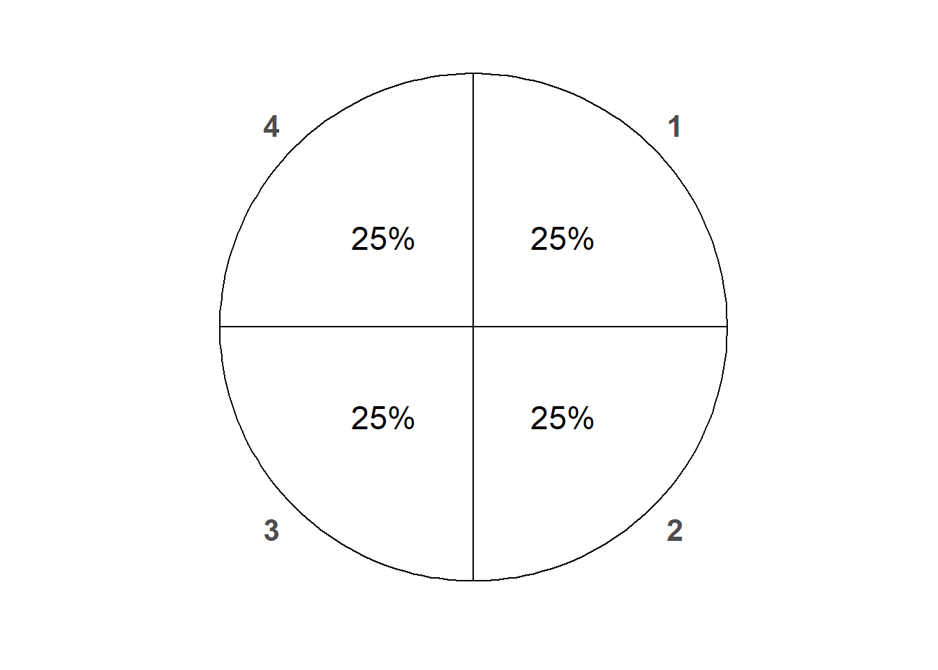
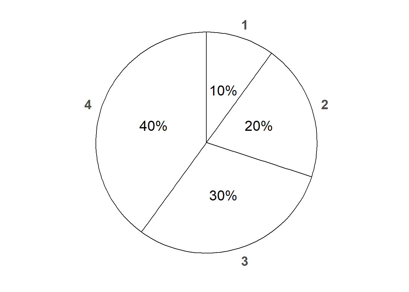
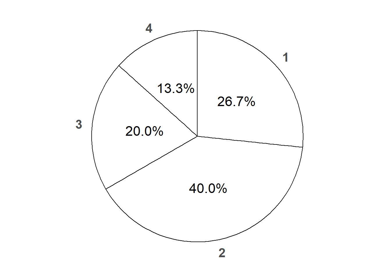
Three possible spinners corresponding to the roll of a four-sided die. Left: a fair die. Middle: the weighted die of Example 2.21. Right: the weighted die of Example 2.22.

Figure 2.6: Three possible spinners corresponding to the roll of a four-sided die. Left: a fair die. Middle: the weighted die of Example 2.21. Right: the weighted die of Example 2.22.

Example 2.23 Roll a four-sided die twice; recall the sample space in Example 2.10 and Table 2.5. One choice of probability measure corresponds to assuming that the die is fair and that the 16 possible outcomes are equally likely. Let $X$ be the sum of the two dice, and let $Y$ be the larger of the two rolls (or the common value if both rolls are the same).

Compute $\textrm{P}(E_1)$, where $E_1$ is the event that the first roll lands on 1.
Compute $\textrm{P}(X = 6)$.
Interpret $\textrm{P}(X = 6)$ as a long run relative frequency.
Interpret $\textrm{P}(X = 6)$ as a relative degree of likelihood. (Hint: compare to $\textrm{P}(X \neq 6)$.)
Construct a table displaying $\textrm{P}(X = x)$ for each possible value $x$ of $X$.
Construct a table displaying $\textrm{P}(Y = y)$ for each possible value $y$ of $Y$.
Construct a table displaying $\textrm{P}(X = x, Y= y)$ for each possible value $(x, y)$ pair.

Solution. to Example 2.23

Show/hide solution

Since $\textrm{P}$ corresponds to equally likely outcomes, we simply need to count the number of outcomes that satisfy the event and divide by the total number of outcomes. There are 16 equally likely outcomes, of which 4 satisfy event $E_1$. (Remember, the sample space corresponds to pairs of rolls, and there are 4 pairs for which the first roll is 1.) So $\textrm{P}(E_1) = 4 / 16 = 1/4$, which makes sense if we’re assuming the die is fair.
There are 16 equally likely outcomes, 3 of which satisfy the event that the sum is 6. So $\textrm{P}(X = 6) = 3 / 16 = 0.1875$.
Over many pairs of rolls of a fair four-sided die, around 18.75% of pairs will yield a sum of 6.
$\textrm{P}(X\neq 6) = 13/16 = 0.8125$. The ratio of $\textrm{P}(X \neq 6)$ to $\textrm{P}(X = 6)$ is $13/3 approx 4.3$. If you roll a fair four-sided die twice, it is 4.3 times more likely for the sum to be something other than 6 than for it to be 6.
The possible values of $X$ are $2, 3, 4, 5, 6, 7, 8$. Find the probability of each value by counting the corresponding outcomes using Table 2.5. For example, $\textrm{P}(X = 3) = \textrm{P}(\{(1, 2), (2, 1)\}) = 2/16$. See Table 2.11.
The possible values of $Y$ are $1, 2, 3, 4$. For example, $\textrm{P}(Y = 3) = \textrm{P}(\{(1, 3), (2, 3), (3, 1), (3, 2), (3, 3)\}) = 5/16$. See table 2.12.
Similar to the previous parts, we can first construct a table with each row corresponding to a possible $(X, Y)$ pair. $\textrm{P}((X, Y) = (4, 3))=\textrm{P}(X = 4, Y=3) = \textrm{P}(\{(1, 3), (3, 1)\}) = 2/16$. See Table 2.13.

Table 2.11: The distribution of $X$, the sum of two rolls of a fair four-sided die.
x	P(X=x)
2	0.0625
3	0.1250
4	0.1875
5	0.2500
6	0.1875
7	0.1250
8	0.0625

Table 2.12: The distribution of $Y$, the larger (or common value if a tie) of two rolls of a fair four-sided die.
y	P(Y=y)
1	0.0625
2	0.1875
3	0.3125
4	0.4375

Table 2.13: Table representing the joint distribution of sum ($X$) and larger ($Y$) of two rolls of a four-sided die
(x, y)	P(X = x, Y = y)
(2, 1)	0.0625
(3, 2)	0.1250
(4, 2)	0.0625
(4, 3)	0.1250
(5, 3)	0.1250
(5, 4)	0.1250
(6, 3)	0.0625
(6, 4)	0.1250
(7, 4)	0.1250
(8, 4)	0.0625

Table 2.14 reorganizes Table 2.13 into a two-way table with rows corresponding to possible values of $X$ and columns corresponding to possible values of $Y$.

Table 2.14: Two-way table representation of the joint distribution of $X$ and $Y$, the sum and the larger (or common value if a tie) of two rolls of a fair four-sided die. Possible values of $X$ are in the leftmost column; possible values of $Y$ are in the top row.
$x$ \ $y$	1	2	3	4
2	1/16	0	0	0
3	0	2/16	0	0
4	0	1/16	2/16	0
5	0	0	2/16	2/16
6	0	0	1/16	2/16
7	0	0	0	2/16
8	0	0	0	1/16

The above tables represent the joint and marginal distributions of the random variables $X$ and $Y$ according to the probability measure $\textrm{P}$, which reflects the assumption that the die is fair and the rolls are independent. The distribution of a random variable describes its possible values and their relative likelihoods. We will study distributions in much more detail as we go.

The distribution of a random variable depends on the underlying probability measure. Changing the probability measure can change the distribution of the random variable. For example, if we used one of the weighted dice from earlier in the sections, the probabilities in the distribution tables for $X$ and $Y$ would change.

Most four-sided dice can reasonably be assumed to be fair, and so the probability models corresponding to the weighted dice in this section might not be very practical. However, remember that most real world situations are not as simple as rolling dice. Just because a situation has 16 possible outcomes doesn’t mean the outcomes have to be equally likely. For example, 16 basketball teams reach the NBA playoffs every year, but that doesn’t mean that all of the 16 playoff teams are equally likely to win the championship.

2.4.2 Some probability measures in the meeting problem

Consider a version of the meeting problem (Example 2.3) where Regina and Cady will definitely arrive between noon and 1, but their exact arrival times are uncertain. Rather than dealing with clock time, it is helpful to represent noon as time 0 and measure time as minutes after noon, so that arrival times take values in the continuous interval [0, 60].

We will use pictures to represent a few probability measures corresponding to different assumptions about the arrival times. In the pictures below, lighter colors represent regions of outcomes that are more likely; darker colors, less likely.

Figure 2.7 corresponds to a “uniform” probability measure under which all outcomes are “equally likely”. This probability measure would be appropriate if we assume that Regina and Cady each arrive at a time uniformly at random between noon and 1, independently of each other.

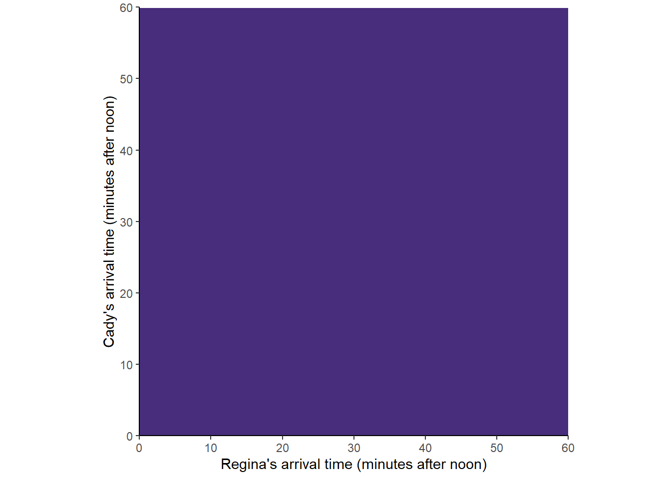
Figure 2.7: A uniform probability measure in the meeting problem

For a finite sample space with equally likely outcomes, computing the probability of an event reduces to counting the number of outcomes that satisfy the event. The continuous analog of equally likely outcomes is a uniform probability measure. When the sample space is uncountable, size is measured continuously (length, area, volume) rather that discretely (counting).

\[ \textrm{P}(A) = \frac{|A|}{|\Omega|} = \frac{\text{size of } A}{\text{size of } \Omega} \qquad \text{if $\textrm{P}$ is a uniform probability measure} \]

Example 2.24 In the meeting problem, assume the uniform probability measure $\textrm{P}$ represented by Figure 2.7.

Find the probability that Regina arrives after Cady.
Find the probability that either Regina or Cady arrives before 12:30.
Find the probability that Cady arrives first and Regina arrives at most 15 minutes after Cady.
Find the probability that Regina arrives before 12:24.
Find the probability that Cady arrive first and Regina arrives at most 1 minute after Cady.
Find the probability that Cady arrives first and Regina arrives at most 1 second after.
Find the probability that Regina and Cady arrive at exactly the same time, with infinite precision.

Solution. to Example 2.24

Show/hide solution

See Figure 2.8 for pictures. Since the sample space is $[0, 60]\times[0, 60]$, a continuous two-dimensional region, “size” is measured by area. Let $\textrm{P}$ be the uniform probability measure on $[0, 60]\times [0, 60]$. The sample space has area 3600. The triangular region corresponding to the event that Regina arrives after Cady has area 3600/2 = 1800. So the probability that Regina arrives after Cady is $1800/3600=0.5$.
The L-shaped region corresponding to the event that Regina or Cady arrives before 12:30 has area $(0.75)(3600)$, so the probability is 0.75.
The trapezoidal region corresponding to the event that that Regina arrives at most 15 minutes after Cady (and Cady arrives first) has area $(7/32)(3600) = (0.21875)(3600)$. (It’s easiest to find the area of the two unshaded triangles and subtract from the total area of 3600: $3600 - 0.5(3600) - (3600)(1-0.25)^2/2=7/32(3600)$.) So the probability that Regina arrives at most 15 minutes after Cady (and Cady arrives first) is 0.21875.
The rectangular region corresponding to the event that that Regina arrives before 12:24 has area (0.4)(3600), so the probability is 0.4.
Similar to part 3, the probability that Regina arrives at most 1 minute after Cady (and Cady arrives first) is $1 - 0.5 - (1-1/60)^2/2=0.0165$.
Similar to part 3, the probability that Regina arrives at most 1 second after Cady (and Cady arrives first) is $1 - 0.5 - (1-1/3600)^2/2=0.000278$.
The event that Regina and Cady arrive at exactly the same time, with infinite precision, corresponds to the “Regina = Cady” line segment. The area of this line segment is 0, so the probability that Regina and Cady arrive at exactly the same time, with infinite precision, is 0.

$Illustration of the events in Exercise 2.24. The square represents the sample space $\Omega=[0,60]\times[0,60]$. With a uniform probability measure, the areas of the shaded regions relative to the whole represent their probabilities.$

Figure 2.8: Illustration of the events in Exercise 2.24. The square represents the sample space $\Omega=[0,60]\times[0,60]$. With a uniform probability measure, the areas of the shaded regions relative to the whole represent their probabilities.

The latter parts of Example 2.24 illustrate that continuous probability spaces introduce some complications that we didn’t encounter when dealing with discrete probability spaces. Regardless of the precise time in the continuous interval $[0, 60]$ at which Regina arrives, the probability that Cady arrives at that exact time, with infinite precision, is 0. We will investigate related ideas in much more detail as we go.

Example 2.25 Continuing Example 2.24, let $R$ be the random variable representing Regina’s arrival time in $[0, 60]$, and $Y$ for Cady. Recall that the random variable $W = |R - Y|$ represents the amount of time the first person to arrive waits for the second person to arrive. The possible values of $W$ lie in the interval $[0, 60]$.

Find and interpret $\textrm{P}(W < 15)$. (Hint: draw a picture representing the event in terms of the pairs of arrival times.)
Find and interpret $\textrm{P}(W > 45)$.
Do the values of $W$ have a “uniform distribution” throughout the interval $[0, 60]$? Explain.

Solution. to Example 2.25

Show/hide solution

The event corresponding to $W<15$ is depicted on the left in Figure 2.9. If Cady arrives first ($R>Y$, below the diagonal in the plot) then $W=R-Y$ so $W<15$ if $R -15 < Y$. If Regina arrives first ($R<Y$, above the diagonal in the plot) then $W=Y-R$ so $W<15$ if $Y < R + 15$. Putting the two cases together $W<15$ if $R - 15 < Y < R + 15$; the corresponding region of $(R, Y)$ pairs is shaded in the plot. According to the uniform probability measure on $[0, 60]\times[0,60]$, $\textrm{P}(W <15)$ is the area of the shaded region (divided by the area of the sample space which is 1). The area of the shaded region is 0.4375(3600). (It is easiest to find the areas of the unshaded triangles and subtract from the total area, $3600(1 - 0.75^2/2 - 0.75^2/2)$.) So $\textrm{P}(W < 15)=0.4375$ is the probability that Regina and Cady arrive within 15 minutes of each other.
The event corresponding to $W>45$ is depicted on the right in Figure 2.9. The probability is the area of the shaded region. So $\textrm{P}(W > 45)=0.25^2/2 + 0.25^2/2=0.0625$ is the probability that Regina and Cady arrive more than 45 minutes apart.
The values of $W$ are not uniformly distributed over $[0, 60]$. For uniform probability measures, regions of the same size have the same probability. But the probability that $W$ lies in the interval $[0, 15]$ is seven times greater than the probability that $W$ lies in the interval $[45, 60]$, even though these intervals have the same length.

$Illustration of the events in Example 2.25. The square represents the sample space $[0,60]\times[0,60]$.$ $Illustration of the events in Example 2.25. The square represents the sample space $[0,60]\times[0,60]$.$

Figure 2.9: Illustration of the events in Example 2.25. The square represents the sample space $[0,60]\times[0,60]$.

Most random phenomenon do not involve equally likely outcomes or uniform probability measures. Even when the underlying outcomes are equally likely, the values of related random variables are usually not. Therefore, most interesting probability problems involve “non-uniform” probability measures.

Figure 2.10 corresponds to one non-uniform probability measure for the meeting problem; certain outcomes are more likely than others. (Lighter colors represent regions of outcomes that are more likely; darker colors, less likely.) Such a probability measure would be appropriate if we assume that Regina and Cady each are more likely to arrive around 12:30 than noon or 1:00, independently of each other.

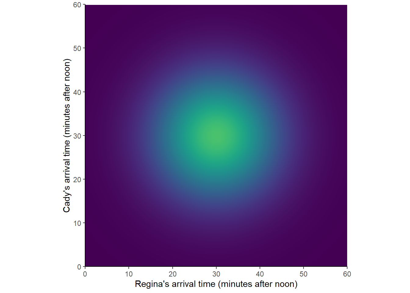
Figure 2.10: A non-uniform probability measure in the meeting problem

Switching from the uniform probability measure represented by Figure 2.7 to the non-uniform one represented by Figure 2.10 would change the probability of the events in Examples 2.24 and 2.25. (We’ll see how to compute probabilities like this later.)

Figure 2.11 corresponds to another “non-uniform” probability measure. Such a probability measure would be appropriate if we assume that Regina and Cady each are more likely to arrive around 12:30 than noon or 1:00, but they coordinate their arrivals so they are more likely to arrive around the same time.

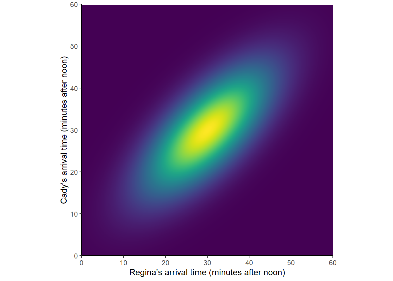
Figure 2.11: Another probability measure in the meeting problem

Figures 2.7, 2.10, and 2.11 represent three different sets of assumptions, and three different probability measures, for the meeting problem. There are many other models. Each probability measure assigns a probability to events like “Cady arrives first”, “both arrive before 12:20”, and “the first person to arrive has to wait less than 15 minutes for the second to arrive”, and these probabilities can differ between models.

Of course, we are leaving out many details behind Figures 2.7, 2.10, and 2.11. We will see later where probability measures like those represented by the pictures above come from, and how to use them. But the pictures illustrate that there can be many assumed probability models for a single situation. There will be many probability measures that satisfy the logical consistency requirements of the probability axioms. Which one is most appropriate depends on the assumptions you make about the random phenomenon.

Perhaps the concept of multiple potential probability measures is easier to understand in a subjective probability situation. For example, each model that is used to forecast the 2022-2023 NFL season corresponds to a probability measure which assigns probabilities to events like “the Eagles win the 2023 Superbowl”. Different sets of assumptions and models can assign different probabilities for the same events. As another example, the weather forecaster on one local news station might report that the probability of rain tomorrow is 0.6, while an online source might report it as 0.5. Each weather forecasting model corresponds to a different probability measure which encodes a set of assumptions about the random phenomenon.

Before moving on, we want to reiterate: Most random phenomenon do not involve equally likely outcomes or uniform probability measures. Even when the underlying outcomes are equally likely, the values of related random variables are usually not. Equally like outcomes or uniform probability measures are the simplest probability measures, and therefore are the ones we typically encounter first. But don’t let that fool you; most interesting probability problems involve non-equally likely outcomes or non-uniform probability measures.

2.4.3 Summary

A probability measure $\textrm{P}$ assigns probabilities to events to quantify their relative likelihoods according to the assumptions of the model of the random phenomenon.
A valid probability measure $\textrm{P}$ must satisfy the following three “axioms”.
- For any event $A$, $0 \le \textrm{P}(A) \le 1$.
- If $\Omega$ represents the sample space then $\textrm{P}(\Omega) = 1$.
- (Countable additivity.) If $A_1, A_2, A_3, \ldots$ are disjoint then \[ \textrm{P}(A_1 \cup A_2 \cup A_2 \cup \cdots) = \textrm{P}(A_1) + \textrm{P}(A_2) +\textrm{P}(A_3) + \cdots \]
Additional properties of a probability measure follow from the axioms
- Complement rule. For any event $A$, $\textrm{P}(A^c) = 1 - \textrm{P}(A)$.
- Subset rule. If $A \subseteq B$ then $\textrm{P}(A) \le \textrm{P}(B)$.
- Addition rule for two events. If $A$ and $B$ are any two events \[\begin{align*} \textrm{P}(A\cup B) = \textrm{P}(A) + \textrm{P}(B) - \textrm{P}(A \cap B) \end{align*}\]
- Law of total probability. If $C_1, C_2, C_3\ldots$ are disjoint events with $C_1\cup C_2 \cup C_3\cup \cdots =\Omega$, then \[\begin{align*} \textrm{P}(A) & = \textrm{P}(A \cap C_1) + \textrm{P}(A \cap C_2) + \textrm{P}(A \cap C_3) + \cdots \end{align*}\]
A probability model (or probability space) is the collection of all outcomes, events, and random variables associated with a random phenomenon along with the probabilities of all events of interest under the assumptions of the model.
The axioms of a probability measure are minimal logical consistent requirements that ensure that probabilities of different events fit together in a valid, coherent way.
A single probability measure corresponds to a particular set of assumptions about the random phenomenon.
There can be many probability measures defined on a single sample space, each one corresponding to a different probability model for the random phenomenon.
Probabilities of events can change if the probability measure changes.

$\Omega$ is the uppercase Greek letter “Omega”. There is no one set of universally agreed on notation, but $\Omega$ is commonly used to represent a sample space. It is also common practice to use uppercase and lowercase letters to denote different objects. The lowercase $\omega$ (lowercase Greek “omega”) is typically used to denote a generic outcome in the sample space. That is, $\Omega$ represents the collection of all the possible outcomes, and $\omega$ represents a particular or generic single outcome.↩︎
Recall that events $A_1, A_2. A_3, \ldots$ are disjoint (a.k.a. mutually exclusive) if they have no outcomes in common; that is, if $A_i \cap A_j = \emptyset$ for all $i\neq j$. Roughly, disjoint events do not “overlap”.↩︎
It’s the number of events that must be countable. The events themselves can be uncountable sets like intervals.↩︎
Proof: Since $\Omega = A \cup A^c$ and $A$ and $A^c$ are disjoint the axioms imply that $1=\textrm{P}(\Omega) = \textrm{P}(A \cup A^c) = \textrm{P}(A) + \textrm{P}(A^c)$.↩︎
Proof. If $A \subseteq B$ then $B = A \cup (B \cap A^c)$. Since $A$ and $(B \cap A^c)$ are disjoint, $\textrm{P}(B) = \textrm{P}(A) + \textrm{P}(B \cap A^c) \ge \textrm{P}(A)$.↩︎
The proof is easiest to see by considering a picture like the one in Figure 2.5 .↩︎
For three events, \[\begin{align*} \textrm{P}(A\cup B\cup C) & = \textrm{P}(A) + \textrm{P}(B) + \textrm{P}(C)\\ & \qquad - \textrm{P}(A\cap B) - \textrm{P}(A \cap C) - \textrm{P}(B \cap C)\\ & \qquad + \textrm{P}(A \cap B \cap C). \end{align*}\]↩︎
That the probability of each outcome must be 1/4 when there are four equally likely outcomes follows from the axioms, by writing $\{1, 2, 3, 4\} = \{1\}\cup\{2\}\cup \{3\}\cup \{4\}$, a union of disjoint sets, and applying countable additivity and $\textrm{P}(\Omega)=1$.↩︎
Probabilities are always defined for events (sets). When we say loosely “the probability of an outcome $\omega$’’ we really mean the probability of the event consisting of the single outcome $\{\omega\}$. In this example $\textrm{P}(\{1\})=\textrm{P}(\{2\})=\textrm{P}(\{3\})=\textrm{P}(\{4\})=1/4$.↩︎

Event	Description	Probability of event assuming equally likely outcomes
\(\emptyset\)	Roll nothing (not possible)	0
\(\{1\}\)	Roll a 1	1/4
\(\{2\}\)	Roll a 2	1/4
\(\{3\}\)	Roll a 3	1/4
\(\{4\}\)	Roll a 4	1/4
\(\{1, 2\}\)	Roll a 1 or a 2	2/4
\(\{1, 3\}\)	Roll a 1 or a 3	2/4
\(\{1, 4\}\)	Roll a 1 or a 4	2/4
\(\{2, 3\}\)	Roll a 2 or a 3	2/4
\(\{2, 4\}\)	Roll a 2 or a 4	2/4
\(\{3, 4\}\)	Roll a 3 or a 4	2/4
\(\{1, 2, 3\}\)	Roll a 1, 2, or 3 (a.k.a. do not roll a 4)	3/4
\(\{1, 2, 4\}\)	Roll a 1, 2, or 4 (a.k.a. do not roll a 3)	3/4
\(\{1, 3, 4\}\)	Roll a 1, 3, or 4 (a.k.a. do not roll a 2)	3/4
\(\{2, 3, 4\}\)	Roll a 2, 3, or 4 (a.k.a. do not roll a 1)	3/4
\(\{1, 2, 3, 4\}\)	Roll something	1

\(x\) \ \(y\)	1	2	3	4
2	1/16	0	0	0
3	0	2/16	0	0
4	0	1/16	2/16	0
5	0	0	2/16	2/16
6	0	0	1/16	2/16
7	0	0	0	2/16
8	0	0	0	1/16