5.6 Conditional expected value
Conditioning on the value of a random variable \(X\) in general changes the distribution of another random variable \(Y\). If a distribution changes, its summary characteristics like expected value and variance can change too.
Example 5.37 Roll a fair four-sided die twice. Let \(X\) be the sum of the two rolls, and let \(Y\) be the larger of the two rolls (or the common value if a tie). We found the joint and marginal distributions of \(X\) and \(Y\) in Example 2.23, displayed in the table below.
| \(p_{X, Y}(x, y)\) | |||||
|---|---|---|---|---|---|
| \(x\) \ \(y\) | 1 | 2 | 3 | 4 | \(p_{X}(x)\) |
| 2 | 1/16 | 0 | 0 | 0 | 1/16 |
| 3 | 0 | 2/16 | 0 | 0 | 2/16 |
| 4 | 0 | 1/16 | 2/16 | 0 | 3/16 |
| 5 | 0 | 0 | 2/16 | 2/16 | 4/16 |
| 6 | 0 | 0 | 1/16 | 2/16 | 3/16 |
| 7 | 0 | 0 | 0 | 2/16 | 2/16 |
| 8 | 0 | 0 | 0 | 1/16 | 1/16 |
| \(p_Y(y)\) | 1/16 | 3/16 | 5/16 | 7/16 |
- Find \(\textrm{E}(Y)\). How could you find a simulation-based approximation?
- Find \(\textrm{E}(Y|X=6)\). How could you find a simulation-based approximation?
- Find \(\textrm{E}(Y|X=5)\). How could you find a simulation-based approximation?
- Find \(\textrm{E}(Y|X=x)\) for each possible value of \(x\) of \(X\).
- Find \(\textrm{E}(X|Y = 4)\). How could you find a simulation-based approximation?
- Find \(\textrm{E}(X|Y = y)\) for each possible value \(y\) of \(Y\).
Solution. to Example 5.37
Show/hide solution
\(\textrm{E}(Y) = 1(1/16) + 2(3/16) + 3(5/16) + 4(7/16) = 3.125\). Approximate this long run average value by simulating many values of \(Y\) and computing the average.
The conditional pmf of \(Y\) given \(X=6\) places probability 2/3 on the value 4 and 1/3 on the value 3. Compute the expected value using this conditional distribution: \(\textrm{E}(Y|X=6) = 3(1/3) + 4(2/3) = 3.67\). This conditional long run average value could be approximated by simulating many \((X, Y)\) pairs from the joint distribution, discarding the pairs for which \(X\neq 6\), and computing the average value of the \(Y\) values for the remaining pairs.
The conditional pmf of \(Y\) given \(X=5\) places probability 1/2 on the value 4 and 1/2 on the value 3. Compute the expected value using this conditional distribution: \(\textrm{E}(Y|X=5) = 3(1/2) + 4(1/2) = 3.5\). This conditional long run average value could be approximated by simulating many \((X, Y)\) pairs from the joint distribution, discarding the pairs for which \(X\neq 5\), and computing the average value of the \(Y\) values for the remaining pairs.
Proceed as in the previous two parts. Find \(\textrm{E}(Y|X=x)\) for each possible value of \(x\) of \(X\).
\(x\) \(\textrm{E}(Y|X=x)\) 2 1(1) = 1 3 2(1) = 2 4 2(1/3) + 3(2/3) = 8/3 5 3(1/2) + 4(1/2) = 3.5 6 3(1/3) + 4(2/3) = 11/3 7 4(1) = 4 8 4(1) = 4 The conditional pmf of \(X\) given \(Y=4\) places probability 2/7 on each of the values 5, 6, 7, and 1/7 on the value 8. Compute the expected value using this conditional distribution: \(\textrm{E}(X|Y=4) = 5(2/7) + 6(2/7) +7(2/7) + 8(1/7)= 6.29\). This conditional long run average value could be approximated by simulating many \((X, Y)\) pairs from the joint distribution, discarding the pairs for which \(Y\neq 4\), and computing the average value of the \(X\) values for the remaining pairs.
Proceed as in the previous part.
\(y\) \(\textrm{E}(X|Y=y)\) 1 2(1) = 2 2 3(2/3) + 4(1/3) = 10/3 3 4(2/5) + 5(2/5) + 6(1/5) = 4.8 4 5(2/7) + 6(2/7) +7(2/7) + 8(1/7) = 44/7
U1, U2 = RV(DiscreteUniform(1, 4) ** 2)

X = U1 + U2

Y = (U1 & U2).apply(max)

y_given_Xeq6 = (Y | (X == 6) ).sim(3000)

y_given_Xeq6| Index | Result |
|---|---|
| 0 | 4 |
| 1 | 3 |
| 2 | 3 |
| 3 | 4 |
| 4 | 4 |
| 5 | 4 |
| 6 | 3 |
| 7 | 3 |
| 8 | 4 |
| ... | ... |
| 2999 | 3 |
y_given_Xeq6.tabulate()| Value | Frequency |
|---|---|
| 3 | 995 |
| 4 | 2005 |
| Total | 3000 |
y_given_Xeq6.mean()## 3.6683333333333334Definition 5.7 The conditional expected value (a.k.a. conditional expectation a.k.a. conditional mean), of a random variable \(Y\) given the event \(\{X=x\}\), defined on a probability space with measure \(\textrm{P}\), is a number denoted \(\textrm{E}(Y|X=x)\) representing the probability-weighted average value of \(Y\), where the weights are determined by the conditional distribution of \(Y\) given \(X=x\).
\[\begin{align*} & \text{Discrete $X, Y$ with conditional pmf $p_{Y|X}$:} & \textrm{E}(Y|X=x) & = \sum_y y p_{Y|X}(y|x)\\ & \text{Continuous $X, Y$ with conditional pdf $f_{Y|X}$:} & \textrm{E}(Y|X=x) & =\int_{-\infty}^\infty y f_{Y|X}(y|x) dy \end{align*}\]
Remember, when conditioning on \(X=x\), \(x\) is treated as a fixed constant. The conditional expected value \(\textrm{E}(Y | X=x)\) is a number representing the mean of the conditional distribution of \(Y\) given \(X=x\). The conditional expected value \(\textrm{E}(Y | X=x)\) is the long run average value of \(Y\) over only those outcomes for which \(X=x\). To approximate \(\textrm{E}(Y|X = x)\), simulate many \((X, Y)\) pairs, discard the pairs for which \(X\neq x\), and average the \(Y\) values for the pairs that remain.
Example 5.38 Recall Example 4.42. Consider the probability space corresponding to two spins of the Uniform(1, 4) spinner and let \(X\) be the sum of the two spins and \(Y\) the larger to the two spins (or the common value if a tie).
- Find \(\textrm{E}(X | Y = 3)\).
- Find \(\textrm{E}(X | Y = 4)\).
- Find \(\textrm{E}(X | Y = y)\) for each value \(y\) of \(Y\).
- Find \(\textrm{E}(Y | X = 3.5)\).
- Find \(\textrm{E}(Y | X = 6)\).
- Find \(\textrm{E}(Y | X = x)\) for each value \(x\) of \(X\).
Solution. to Example 5.38
Show/hide solution
- Recall Figure 4.42. All the conditional distributions (slices) are Uniform, but over different ranges of possible values. Remember, the mean of any Uniform distribution is the midpoint of the possible range of values. The conditional distribution of \(X\) given \(Y=3\) is the Uniform(4, 6) distribution, which has mean 5. Therefore, \(\textrm{E}(X | Y = 3)=5\). As an integral, since \(f_{X|Y}(x|3) = 1/2, 4<x<6\), \[ \textrm{E}(X | Y = 3) = \int_4^6 x (1/2)dx = \frac{x^2}{4}\Bigg|_{x=4}^{x=6} = \frac{6^2}{4} - \frac{4^2}{4} = 5. \]
- The conditional distribution of \(X\) given \(Y=4\) is the Uniform(5, 8) distribution, which has mean 6.5. Therefore, \(\textrm{E}(X | Y = 4)=6.5\).
- For a given \(y\), the conditional distribution of \(X\) given \(Y=y\) is the Uniform(\(y+1\), \(2y\)) distribution, which has mean \(\frac{y+1+2y}{2}=1.5y + 0.5\). Therefore, \(\textrm{E}(X | Y = y)=1.5y + 0.5\). As an integral, since \(f_{X|Y}(x|y) = \frac{1}{y-1}, y+1 < x< 2y\), \[ \textrm{E}(X | Y = y) = \int_{y+1}^{2y} x \left(\frac{1}{y-1}\right)dx = \frac{x^2}{2(y-1)}\Bigg|_{x=y+1}^{x=2y} = \frac{(2y)^2}{2(y-1)} - \frac{(y+1)^2}{2(y-1)} = 1.5y + 0.5. \] In the above, \(y\) is treated like a fixed constant, and we are averaging over values of \(X\) by taking a \(dx\) integral. For a given value of \(y\) like \(y=3\), \(1.5y + 0.5\) is a number like \(1.5(3)+0.5=5\).
- The conditional distribution of \(Y\) given \(X=3.5\) is the Uniform(1.75, 2.5) distribution, which has mean 2.125. Therefore, \(\textrm{E}(Y | X = 3.5)=2.125\). As an integral, since \(f_{Y|X}(y|3.5) = 1/0.75, 1.75<y<2.5\), \[ \textrm{E}(Y | X = 3.5) = \int_{1.75}^{2.5} y (1/0.75)dy = \frac{y^2}{1.5}\Bigg|_{y=1.75}^{y=2.5} = \frac{2.5^2}{1.5} - \frac{1.75^2}{1.5} = 2.125. \]
- The conditional distribution of \(Y\) given \(X=6\) is the Uniform(3, 4) distribution, which has mean 3.5. Therefore, \(\textrm{E}(Y | X = 6)=3.5\).
- There are two general cases. If \(2<x<5\) then the conditional distribution of \(Y\) given \(X=x\) is Uniform(\(0.5x\), \(x-1\)) so \(\textrm{E}(Y|X = x) = \frac{0.5x + x - 1}{2} = 0.75x - 0.5\). If \(5<x<8\) then the conditional distribution of \(Y\) given \(X=x\) is Uniform(\(0.5x\), 4) so \(\textrm{E}(Y|X = x) = \frac{0.5x + 4}{2} = 0.25x +2\). The two cases can be put together as \[ \textrm{E}(Y | X = x) = 0.25x + 0.5\min(4, x-1). \] In the above, \(x\) is treated like a fixed constant, and we are averaging over values of \(Y\) by taking a \(dy\) integral. For a given value of \(x\) like \(x=3.5\), \(0.25x + 0.5\min(4, x-1)\) is a number like \(0.25(3.5) + 0.5\min(4, 3.5-1)=2.125\).
Remember that the probability that a continuous random variable is equal to a particular value is 0; that is, for continuous \(X\), \(\textrm{P}(X=x)=0\). When we condition on \(\{X=x\}\) we are really conditioning on \(\{|X-x|<\epsilon\}\) and seeing what happens in the idealized limit when \(\epsilon\to0\).
When simulating, never condition on \(\{X=x\}\) for a continuous random variable \(X\); rather, condition on \(\{|X-x|<\epsilon\}\) where \(\epsilon\) represents some suitable degree of precision (e.g. \(\epsilon=0.005\) if rounding to two decimal places).
To approximate \(\textrm{E}(Y|X = x)\) for continuous random variables, simulate many \((X, Y)\) pairs, discard the pairs for which \(X\) is not close to \(x\), and average the \(Y\) values for the pairs that remain.
U1, U2 = RV(Uniform(1, 4) ** 2)

X = U1 + U2

Y = (U1 & U2).apply(max)

x_given_Yeq3 = (X | (abs(Y - 3) < 0.05) ).sim(1000)

x_given_Yeq3| Index | Result |
|---|---|
| 0 | 5.4825136229456195 |
| 1 | 4.285458771011861 |
| 2 | 4.979280857973896 |
| 3 | 5.227358857091753 |
| 4 | 5.3544112730493385 |
| 5 | 4.776259497735202 |
| 6 | 5.7442736208405005 |
| 7 | 5.901424378706625 |
| 8 | 5.897231760125052 |
| ... | ... |
| 999 | 5.697754319932682 |
x_given_Yeq3.plot()
plt.show()
x_given_Yeq3.mean()## 4.9908204399220845.6.1 Conditional expected value as a random variable
Given a value \(x\) of \(X\), the conditional expected value \(\textrm{E}(Y|X=x)\) is a number. However, since \(X\) can take different values \(x\), then \(\textrm{E}(Y|X=x)\) can also take different values depending on the value of \(x\). That is, \(\textrm{E}(Y|X=x)\) is a function of \(x\). Moreover, since \(X\) is a random variable, \(\textrm{E}(Y|X=x)\) is a function of values of a random variable.
Example 5.39 Recall Example 2.63. In the meeting problem, assume that \(R\) follows a Normal(30, 10) distribution. For any value \(r\), assume that the conditional distribution of \(Y\) given \(R=r\) is a Normal distribution with mean \(30 + 0.7(r - 30)\) and standard deviation 7.14 minutes.
- Compute and interpret \(\textrm{E}(Y| R = 40)\).
- Compute and interpret \(\textrm{E}(Y| R = 15)\).
- Provide an expression for \(\textrm{E}(Y|R)\).
- Identify the distribution of the random variable \(E(Y|R)\).
- Explain in words in context what the distribution in the previous part represents.
Solution. to Example 5.39
Show/hide solution
- The assumed conditional distribution of \(Y\) given \(R=40\) is Normal with mean \(30 + 0.7(40 - 30) = 37\) and standard deviation 7.14 minutes. The mean of this distribution is 37. Therefore \(\textrm{E}(Y | R = 40) = 37\). Over many days where Regina arrives 40 minutes after noon, Cady’s conditional average arrival time is 37 minutes after noon.
- The assumed conditional distribution of \(Y\) given \(R=15\) is Normal with mean \(30 + 0.7(15 - 30) = 19.5\) and standard deviation 7.14 minutes. The mean of this distribution is 19.5. Therefore \(\textrm{E}(Y | R) = 19.5\). Over many days where Regina arrives 15 minutes after noon, Cady’s conditional average arrival time is 19.5 minutes after noon.
- The assumed conditional distribution of \(Y\) given \(R=r\) is Normal with mean \(30 + 0.7(r - 30)\) and standard deviation 7.14 minutes. The mean of this distribution is \(30 + 0.7(r - 30)\). Therefore \(\textrm{E}(Y | R = r) = 30 + 0.7(r - 30)\); in this expression, \(r\) represents a particular number (like 40 or 15). Regardless of Regina’s arrival time, Cady’s conditional average arrival time is given by \(\textrm{E}(Y | R) = 30 + 0.7(R - 30)\); notice that this is a function of the random variable \(R\).
- \(\textrm{E}(Y | R) = 30 + 0.7(R - 30)\) is a linear rescaling of \(R\). Since \(R\) has a Normal distribution, any linear rescaling of \(R\) also has a Normal distribution. The mean is \(30 + 0.7(\textrm{E}(R) - 30) = 30 + 0.7(30-30) = 30\) minutes after noon and the standard deviation is \(0.7(\textrm{SD}(R)) = 0.7(10) = 7\) minutes after noon. That is, \(\textrm{E}(Y | R) = 30 + 0.7(R - 30)\) has a Normal(30, 7) distribution.
- See below.
Consider Figure 5.6 which represents the situation in Example 5.39. The orange vertical slices represent the conditional distribution of \(Y\) given \(R=r\) for \(r = 10, 15, 20, \ldots, 45, 50\). The pink dots in the center of the slices represent the conditional averages, \(\textrm{E}(Y|R = r)\) for the different values of \(r\). The pink line connecting the conditional averages represents \(\textrm{E}(Y | R) = 30 + 0.7(R - 30)\).
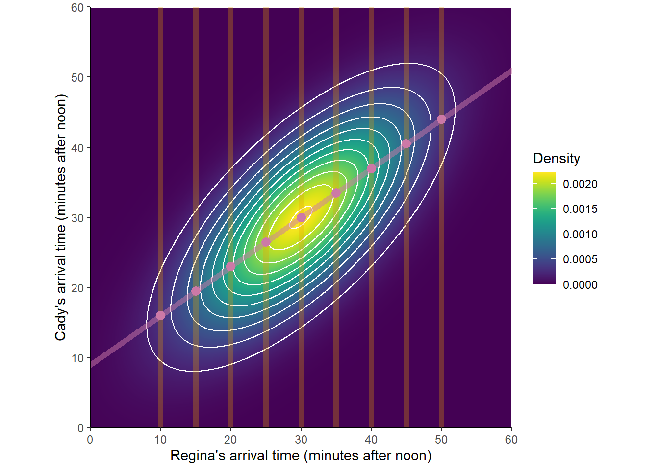
Figure 5.6: A Bivariate Normal distribution with some conditional distributions and conditional expected values highlighted.
In the previous example, suppose that every day when Regina arrives she guesses what time Cady arrived/will arrive that day (if Regina arrives second/first). Suppose each day Regina’s guess is equal to Cady’s conditional average arrival time given Regina’s arrival time. For example, every day Regina arrives 40 minutes after noon, she guesses Cady’s arrival time is 37 minutes after noon; every day Regina arrives 15 minutes after noon, she guess Cady’s arrival time is 19.5 minutes after noon. Then the distribution of \(\textrm{E}(Y|R)\) represents how Regina’s guesses for Cady’s arrival time would be distributed over a large number of days. The values of \(\textrm{E}(Y|R)\) would be given by \(30 + 0.7(R - 30)\), a function of \(R\). The distribution of values of \(\textrm{E}(Y|R)\) would be determined by the distribution of \(R\). For example, there would be more days where Regina arrives 40 minutes after noon than where she arrives 15 minutes after noon, so guesses of 37 minutes after noon (\(\textrm{E}(Y|R=40)=37\)) would occur more frequently than guesses of 19.5 minutes after noon (\(\textrm{E}(Y|R=15)=19.5\)).
Example 5.40 Continuing Example 5.37. Let \(X\) be the sum of the two rolls, and let \(Y\) be the larger of the two rolls (or the common value if a tie).
- Let \(\ell(x)\) denote the function that maps values \(x\) of \(X\) to \(\textrm{E}(Y|X=x)\). Find the distribution of the random variable \(Z=\ell(X)\).
- Find \(\textrm{P}(Z\le 3)\).
- Let \(\textrm{E}(X|Y)\) denote the random variable that takes value \(\textrm{E}(X|Y=y)\) when \(Y=y\). Find the distribution of \(\textrm{E}(X|Y)\).
- Find \(\textrm{P}(\textrm{E}(X|Y)\le 4)\).
Solution. to Example 5.40
Show/hide solution
We have already found \(\textrm{E}(Y|X=x)\) for each \(x\). The table below defines the function \(\ell\).
\(x\) \(\ell(x) = \textrm{E}(Y|X =x)\) 2 1 3 2 4 8/3 5 3.5 6 11/3 7 4 8 4 The random variable \(Z=\ell(X)\) takes values 1, 2, 8/3, 3.5, 11/3, and 4. Since \(Z\) is a function of \(X\), the distribution of \(Z\) is determined by the distribution of \(X\). For example, \(\textrm{P}(Z = 8/3) = \textrm{P}(X=4) = 3/16\), and \(\textrm{P}(Z = 4) = \textrm{P}(X=7)+\textrm{P}(X = 8)=3/16\). The following table displays the pmf of \(Z\).
\(z\) \(p_Z(z)\) 1 1/16 2 2/16 8/3 3/16 3.5 4/16 11/3 3/16 4 3/16 Use the table above. The possible values of \(Z\) that are at most 3 are 1, 2, 8/3, so \(\textrm{P}(Z\le 3) = 6/16\).
This is similar to the previous parts, but now we are conditioning the other way and using different notation. Let \(w\) denote a generic possible value of the random variable \(\textrm{E}(X|Y)\). The possible values of \(\textrm{E}(X|Y)\) are determined by \(\textrm{E}(X|Y=y)\) for each possible value \(y\) of \(Y\), and the corresponding probabilities are determined by the distribution of \(Y\). The following table displays the pmf of \(\textrm{E}(X|Y)\).
\(w\) \(p_{\textrm{E}(X|Y)}(w)\) 2 1/16 10/3 3/16 4.8 5/16 44/7 7/16 Use the table above. \(\textrm{P}(\textrm{E}(X|Y)\le 4) = 4/16\).
Definition 5.8 The conditional expected value of \(Y\) given \(X\) is the random variable, denoted \(\textrm{E}(Y|X)\), which takes value \(\textrm{E}(Y|X=x)\) on the occurrence of the event \(\{X=x\}\). The random variable \(\textrm{E}(Y|X)\) is a function of \(X\).
For a given value \(x\) of \(X\), \(\textrm{E}(Y|X=x)\) is a number. Let \(\ell\) denote the function which maps \(x\) to the number \(\ell(x)=\textrm{E}(Y|X=x)\). The random variable \(\textrm{E}(Y|X)\) is a function of \(X\), namely \(\textrm{E}(Y|X)=\ell(X)\).
Roughly, \(\textrm{E}(Y|X)\) can be thought of as the “best guess” of the value of \(Y\) given only the information available from \(X\).
Since \(\textrm{E}(Y|X)\) is a random variable, it has a distribution. And since \(\textrm{E}(Y|X)\) is a function of \(X\), the distribution of \(X\) will be depend on the distribution of \(X\). However, remember that a transformation generally changes the shape of a distribution, so the distribution of \(\textrm{E}(Y|X)\) will usually have a different shape than that of \(X\).
Example 5.41 Continuing Example 5.38. Consider the probability space corresponding to two spins of the Uniform(1, 4) spinner and let \(X\) be the sum of the two spins and \(Y\) the larger to the two spins (or the common value if a tie).
- Find an expression for \(\textrm{E}(X | Y)\).
- Find \(\textrm{P}(\textrm{E}(X|Y) \le 5)\).
- Find the pdf of \(\textrm{E}(X|Y)\).
- Find an expression for \(\textrm{E}(Y | X)\).
Solution. to Example 5.41
Show/hide solution
The conditional distribution of \(X\) given \(Y=y\) is Uniform(\(y+1\), \(2y\)) distribution, which has mean \(\frac{y+1+2y}{2}=1.5y + 0.5\). This is true for any value \(y\) of \(Y\). Therefore, \(\textrm{E}(X|Y) = 1.5Y + 0.5\), a function of \(Y\).
Remember that the pdf of \(Y\) is \(f_Y(y) = (2/9)(y-1), 1<y<4\). \[ \textrm{P}(\textrm{E}(X|Y) \le 5) = \textrm{P}(1.5Y + 0.5 \le 5) = \textrm{P}(Y \le 3) = \int_1^3 (2/9)(y-1)dy = 4/9 \]
\(E(X|Y)=1.5Y+0.5\) is a linear transformation of \(Y\), so the shape of its distribution will be the same as the shape of the distribution of \(Y\). The possible values of \(\textrm{E}(X|Y)\) are 2 to 6.5. We can use the cdf method. For \(2<w<6.5\),
\[\begin{align*} F_{\textrm{E}(X|Y)}(w) & = \textrm{P}(\textrm{E}(X|Y)\le w)\\ & = \textrm{P}(1.5Y + 0.5 \le w)\\ & = \textrm{P}(Y \le (w - 0.5)/1.5)\\ F_{\textrm{E}(X|Y)}(w)& = F_Y((w-0.5)/1.5) \end{align*}\]
Differentiate both sides with respect to \(w\); remember the chain rule. \[ f_{\textrm{E}(X|Y)}(w) = f_Y((w-0.5)/1.5)(1/1.5) = (2/9)((w-0.5)/1.5 - 1)/1.5 = (8/81)(w - 2) \]
That is, the pdf of \(\textrm{E}(X|Y)\) is \(f_{\textrm{E}(X|Y)}(w) = (8/81)(w - 2), 2<w<6.5\).
For each \(2<x<8\), \[ \textrm{E}(Y | X = x) = 0.25x + 0.5\min(4, x-1). \] Therefore, \(\textrm{E}(Y | X) = 0.25X + 0.5\min(4, X-1)\), a function of \(X\).
5.6.2 Linearity of conditional expected value
Conditional expected value, whether viewed as a number \(\textrm{E}(Y|X=x)\) or a random variable \(\textrm{E}(Y|X)\), possesses properties analogous to those of (unconditional) expected value. In particular, we have linearity of conditional expected value.
If \(X, Y_1, \ldots, Y_n\) are RVs and \(a_1, \ldots, a_n\) are non-random constants then \[\begin{align*} \textrm{E}(a_1Y_1+\cdots+a_n Y_n|X=x) & = a_1\textrm{E}(Y_1|X=x)+\cdots+a_n\textrm{E}(Y_n|X=x)\\ \textrm{E}(a_1Y_1+\cdots+a_n Y_n|X) & = a_1\textrm{E}(Y_1|X)+\cdots+a_n\textrm{E}(Y_n|X) \end{align*}\] The first line above is an equality involving numbers; the second line is an equality involving random variables (i.e., functions).
Example 5.42 Continuing Example 5.41. Spin the Uniform(1, 4) spinner twice, let \(U_1\) be the result of the first spin, \(U_2\) the second, and let \(X=U_1+U_2\) and \(Y=\max(U_1, U_2)\).
- Use linearity to show \(\textrm{E}(U_1|Y) = 0.75Y + 0.25\).
- Explain intuitively why \(\textrm{E}(U_1|Y) = 0.75Y + 0.25\).
Solution. to Example 5.42
Show/hide solution
- By symmetry, \(\textrm{E}(U_1|Y) = \textrm{E}(U_2|Y)\). By linearity of conditional expected value \[ \textrm{E}(X|Y) = \textrm{E}(U_1 + U_2|Y) = \textrm{E}(U_1|Y) + \textrm{E}(U_2|Y) = 2\textrm{E}(U_1|Y) \] So \(\textrm{E}(U_1|Y) = 0.5\textrm{E}(X|Y) = 0.5(1.5Y + 0.5)=0.75Y + 0.25\).
- Given the larger value \(Y\), there are two cases. Either the first spin is the larger, which happens with probability 0.5, in which case \(U_1=Y\) so \(\textrm{E}(U_1|Y) = Y\). Otherwise, the second spin is the larger, which happens with probability 0.5, in which case \(U_1\) is Uniformly distributed between 1 and \(Y\) with mean \((Y+1)/2\). Therefore, \(\textrm{E}(U_1|Y) = 0.5Y + 0.5(Y+1)/2 = 0.75Y + 0.25\).
5.6.3 Law of total expectation
Analogous to the law of total probability, the law of total expectation provides a way of computing an expected value by breaking down a problem into various cases, computing the conditional expected value given each case, and then computing the overall expected value as a probability-weighted average of these case-by-case conditional expected values.
Example 5.43 Continuing Example 5.40. Let \(X\) be the sum of the two rolls, and let \(Y\) be the larger of the two rolls (or the common value if a tie).
- Find the expected value of the random variable \(\textrm{E}(X|Y)\). That is, find \(\textrm{E}(\textrm{E}(X|Y))\). How does it relate to \(\textrm{E}(X)\)?
- Find the expected value of the random variable \(\textrm{E}(Y|X)\). That is, find \(\textrm{E}(\textrm{E}(Y|X))\). How does it relate to \(\textrm{E}(Y)\)?
Solution. to Example 5.43
Show/hide solution
\(\textrm{E}(X|Y)\) is a discrete random variable with pmf
\(w\) \(p_{\textrm{E}(X|Y)}(w)\) 2 1/16 10/3 3/16 4.8 5/16 44/7 7/16 Therefore, \[ \textrm{E}(\textrm{E}(X|Y)) = (2)(1/16) + (10/3)(3/16) + (4.8)(5/16) + (44/7)(7/16) = 5 \] We see that \(\textrm{E}(\textrm{E}(X|Y)) = 5 = \textrm{E}(X)\).
\(\textrm{E}(Y|X)\) is a discrete random variable with pmf
\(z\) \(p_{\textrm{E}(Y|X)}(z)\) 1 1/16 2 2/16 8/3 3/16 3.5 4/16 11/3 3/16 4 3/16 Therefore, \[ \textrm{E}(\textrm{E}(Y|X)) = (1)(1/16) + (2)(2/16) + (8/4)(3/16) + (3.5)(4/16) +(11/3)(3/16)+(4)(3/16)= 3.125 \] We see that \(\textrm{E}(\textrm{E}(Y|X)) = 3.125 = \textrm{E}(Y)\).
Theorem 5.3 (Law of Total Expectation (LTE)) For any two random variables \(X\) and \(Y\) (defined on the same probability space) \[ \textrm{E}(Y) = \textrm{E}(\textrm{E}(Y|X)) \]
Remember that \(\textrm{E}(Y|X)\) is a random variable and so it has an expected value \(\textrm{E}(\textrm{E}(Y|X))\) representing the long run average value of the random variable \(\textrm{E}(Y|X)\). Also remember that \(\textrm{E}(Y|X)\) is a function of \(X\) and so \(\textrm{E}(\textrm{E}(Y|X))\) can be computed using LOTUS using the distribution of \(X\). For two discrete random variables \(X\) and \(Y\) \[ \textrm{E}(\textrm{E}(Y|X)) = \sum_x \textrm{E}(Y|X=x)p_X(x) \]
Here is a proof of the LTE for discrete random variables. (The proof for continuous random variables is analogous). \[\begin{align*} \textrm{E}(\textrm{E}(Y|X)) & = \sum_x \textrm{E}(Y|X=x)p_X(x) & & \text{LOTUS, $\textrm{E}(Y|X)$ is a function of $X$}\\ & = \sum_x \left(\sum_y y p_{Y|X}(y|x)\right) p_X(x) & & \text{definition of CE}\\ & = \sum_x \sum_y y p_{X, Y}(x, y) & & \text{joint = conditional $\times$ marginal}\\ & = \sum_y y \sum_x p_{X, Y}(x, y) & & \text{interchange sums}\\ & = \sum_y y p_Y(y) & & \text{collapse joint to get marginal}\\ & = \textrm{E}(Y) & & \text{definition of expected value} \end{align*}\]
Example 5.44 Continuing Example 5.41. Consider the probability space corresponding to two spins of the Uniform(1, 4) spinner and let \(X\) be the sum of the two spins and \(Y\) the larger to the two spins (or the common value if a tie).
- Use the distribution of the random variable \(E(X|Y)\) to compute \(\textrm{E}(\textrm{E}(X|Y))\). Compare to \(\textrm{E}(X)\).
- Use the expression for \(\textrm{E}(X|Y)\) and properties of expected value to compute \(\textrm{E}(\textrm{E}(X|Y))\).
Solution. to Example 5.44
Show/hide solution
- The continuous random variable \(\textrm{E}(X|Y)\) has pdf \(f_{\textrm{E}(X|Y)}(w) = (8/81)(w - 2), 2<w<6.5\). So the expected value is \[ \textrm{E}(\textrm{E}(X|Y)) = \int_2^{6.5} w \left((8/81)(w-2)\right)dw = 5 \]
- \(E(X|Y)=1.5Y+0.5\) so \(\textrm{E}(E(X|Y))=\textrm{E}(1.5Y+0.5)=1.5\textrm{E}(Y) + 0.5=1.5(3)+0.5\). We can find \(\textrm{E}(Y)=3\) using its pdf: \(\textrm{E}(Y) = \int_1^4 y (2/9)(y-1)dy = 3\).
Conditioning can be used as a problem solving strategy. Conditioning can be used with the law of total probability to compute unconditional probabilities. Likewise, conditioning can be used with the law of total expectation to compute unconditional expected values.
Example 5.45 Flip a fair coin repeatedly.
- What is the expected value of the number of tosses until a flip lands on H? (Count the tosses that result in H, so H is 1 flip, TH is 2 flips, TTH is 3 flips, etc).
- What is the expected value of the number of flips until you see H followed immediately by T? (HT is 2 flips, HHT is 3 flips, THT is 3 flips, HHHT is 4 flips, etc)
- What is the expected value of the number of flips until you see H followed immediately by H? (HH is 2 flips, THH is 3 flips, HTHH is 4 flips, HTTHH is 5 flips, etc)
- Which of the previous two parts has the larger expected value? Can you explain why?
Solution. to Example 5.45
Show/hide solution
- Let \(\mu\) be the expected value in question. Condition on the result of the first flip. Either the first flip is H, with probability 1/2, in which case you’re done with 1 flip. Otherwise, the first flip is T in which case the process starts over after the first flip and the expected number of additional flips is also \(\mu\). Use the law of total expectation to put the two expected values together. \[ \mu = (1/2)(1) + (1/2)(1+\mu) \] Solve for \(\mu=2\).
- To achieve the pattern HT, we first need to flip until we get H, and then we complete the pattern once we get the first T after that. The expected number of flips until the first H is 2 (from the previous part). By symmetry, the expected number of additional flips until the first T is also 2. By linearity of expected value, the expected value of the number of flips to achieve HT is 4.
- Let \(\mu\) denote the expected value in question. Condition on the result of the first flip. If we get T, we’re right back where we started after 1 flip, and the expected number of additional flips is \(\mu\). If the first flip is H, consider the second flip. If it’s H, then we’re done in 2 flips. If the second flip is T, then after 2 flips we’re back at the beginning again and the expected number of additional flips is \(\mu\). Use the law of total expectation to put it all together. \[ \mu = (1/2)(1 + \mu) + (1/2)((1/2)(2) + (1/2)(2+\mu)) \] Solve to find \(\mu = 6\).
- It takes longer on average to see HH than HT. When trying for HH, any T that follows H destroys our progress and takes us back to the beginning. But when trying for HT, any H that follows H just maintains our current position.
Example 5.46 Recall Example 3.5. You and your friend are playing the “lookaway challenge”. The game consists of possibly multiple rounds. In the first round, you point in one of four directions: up, down, left or right. At the exact same time, your friend also looks in one of those four directions. If your friend looks in the same direction you’re pointing, you win! Otherwise, you switch roles and the game continues to the next round — now your friend points in a direction and you try to look away. (So the player who starts as the pointer is the pointer in the odd-numbered rounds, and the player who starts as the looker is the pointer in the even-numbered rounds, until the game ends.) As long as no one wins, you keep switching off who points and who looks. The game ends, and the current “pointer” wins, whenever the “looker” looks in the same direction as the pointer.
We saw in Example 3.5 that the probability that the player who starts as the pointer wins the game is 4/7 = 0.571.
- Compute and interpret the expected number of rounds in a game.
- Compute and intepret the conditional expected number of rounds in a game given that the player who is the pointer in the first round wins the game.
- Compute and interpret the conditional expected number of rounds in a game given that the player who is the looker in the first round wins the game.
Solution. to Example 5.46
Show/hide solution
- Let \(X\) be the number of rounds in the game. We want \(\mu = \textrm{E}(X)\). Condition on the result of the first round. If the pointer wins the first round, which occurs with probability 1/4, the game is over and \(X=1\). If the pointer does now win the first round, which occurs with probability 3/4, one round is played and then the game “starts over” and the expected number of additional rounds is \(\mu\). By the law of total expectation \(\mu = (1)(1/4) + (1+\mu)(3/4)\); solve for \(\mu = 4\). Over many games, on average 4 rounds are played.
- Let \(I\) be the indicator that the player who starts as the pointer wins the game.
We want \(\mu_1 = \textrm{E}(X|I=1)\).
We can basically repeat our strategy from the previous part, but now we condition on the player who starts as the pointer winning the game everywhere.
Again, we’ll consider two cases based on the results of the first round.
If the pointer wins the first round, the game ends and \(X = 1\); the weight of this case is the conditional probability that the pointer wins in the first round given that the pointer wins the game, which is
\[
\textrm{P}(\text{first pointer wins first round} | \text{first pointer wins game}) = \frac{\textrm{P}(\text{first pointer wins first round and first pointer wins game})}{\textrm{P}(\text{first pointer wins game})} = \frac{1/4}{4/7} = 7/16=0.4375
\]
If the pointer does not win the first round, given that the first pointer wins the game then 2 more rounds are played — given that the first pointer wins the game, the game cannot end in round 2 — and then the game “starts over”.
By the law of total expectation
\[
\mu_1 = (1)(7/16) + (2 + \mu_1)(9/16)
\]
Solve for \(\mu_1 = 25/7 = 3.57\).
Over many games where the player who starts as the pointer wins on average 3.57 rounds are played.
- We might expect the answer to this part to be 32/7, the answer to the previous part plus 1; the previous part is the average number of rounds given that the game ends in an odd number of rounds, and now we want the average number of rounds give that the game ends in an even number of rounds. We want \(\mu_0 = \textrm{E}(X|I=0)\). We can use the results of the previous two parts if we condition on which player wins the game and use the law of total expectation. If the first pointer wins the game, which happens with probability 4/7, the conditional expected value is 25/7. If the first pointer does not win the game, which happens with probability 3/7, the conditional expected value is \(\mu_0\). The overall expected value is 4, so use the law of total expected value \[\begin{align*} \textrm{E}(X) & = \textrm{E}(X|I = 1)\textrm{P}(I = 1) + \textrm{E}(X | I = 0)\textrm{P}(I = 0)\\ 4 & = (25/7)(4/7) + \mu_0(3/7) \end{align*}\] Solve for \(\mu_0 = 32/7 = 4.57\). Over many games where the player who starts as the pointer does not win on average 4.57 rounds are played.
The following is a simulation of the lookaway challenge problem.
def count_rounds(sequence):
    for r, pair in enumerate(sequence):
        if pair[0] == pair[1]:
            return r + 1 # +1 for 0 indexing

P = BoxModel([1, 2, 3, 4], size = 2) ** inf

X = RV(P, count_rounds)

x = X.sim(25000)

x| Index | Result |
|---|---|
| 0 | 1 |
| 1 | 4 |
| 2 | 9 |
| 3 | 10 |
| 4 | 5 |
| 5 | 7 |
| 6 | 2 |
| 7 | 4 |
| 8 | 4 |
| ... | ... |
| 24999 | 4 |
Approximate distribution of the number of rounds.
x.plot()
Approximate probability that the player who starts as the pointer wins the game (which occurs if the game ends in an odd number of rounds).
def is_odd(u):
    return (u % 2) == 1 # odd if the remainder when dividing by 2 is 1

x.count(is_odd) / x.count()
## 0.5714Approximate expected number of rounds.
x.mean()## 3.96004Approximate conditional probability that the player who starts as the pointer wins in the first round given that the player who starts as the pointer wins the game.
x.count_eq(1) / x.count(is_odd)## 0.43633181659082954Approximate conditional expected number of rounds given that the player who starts as the pointer wins the game.
x.filter(is_odd).mean()## 3.5528876443822193Approximate conditional expected number of rounds given that the player who starts as the pointer does not win the game.
def is_even(x):
    return (x % 2) == 0 # odd if the remainder when dividing by 2 is 0

x.filter(is_even).mean()
## 4.50284647690153955.6.4 Taking out what is known
Example 5.47 Suppose you construct a “random rectangle” as follows. The base \(X\) is a random variable with a Uniform(0, 1) distribution. The height \(Y\) is a random variable whose conditional distribution given \(X=x\) is Uniform(0, \(x\)). We are interested in \(\textrm{E}(Y)\) the expected value of the height of the rectangle.
- Explain how you could use the Uniform(0, 1) spinner to simulate an \((X, Y)\) pair.
- Explain how you could use simulation to approximate \(\textrm{E}(Y)\).
- Find \(\textrm{E}(Y|X=0.5)\).
- Find \(\textrm{E}(Y|X=0.2)\).
- Find \(\textrm{E}(Y|X=x)\) for a generic \(x\in(0, 1)\).
- Identify the random variable \(\textrm{E}(Y|X)\).
- Use LTE to find \(\textrm{E}(Y)\).
- Sketch a plot of the joint distribution of \((X, Y)\).
- Sketch a plot of the marginal distribution of \(Y\). Be sure to specify the possible values. Is it Uniform?
- What would you need to do to find \(\textrm{E}(Y)\) using the definition of expected value?
Solution. to Example 5.47
- Spin the spinner twice and let \(U_1\) be the result of the first spin and \(U_2\) the result of the second. Let \(X=U_1\). Now consider an example. Given \(X=0.2\), we want \(Y\) to have a Uniform(0, 0.2) distribution. So we could take the result of the second spin (on a (0, 1) scale) and multiply by 0.2 to get a value on a (0, 0.2) scale. (Remember: linear rescaling only changes the possible values and not the shape of the distribution; see Section 2.8.3.) That is, conditional on \(X=0.2\), \(0.2U_2\) will have a Uniform(0, 0.2) distribution. Conditional on a general \(x\), \(xU_2\) will have a Uniform(0, \(x\)) distribution. So if we define the random variable \(Y\) as \(Y=XU_2\), then the conditional distribution of \(Y\) given \(X=x\) will be Uniform(0, \(x\)).
- Simulate many \((X, Y)\) pairs in the above manner, and find the average of the simulated \(Y\) values to approximate \(\textrm{E}(Y)\).
- The conditional distribution of \(Y\) given \(X=0.5\) is Uniform(0, 0.5) so \(\textrm{E}(Y|X=0.5)=0.5/2 = 0.25\).
- The conditional distribution of \(Y\) given \(X=0.2\) is Uniform(0, 0.2) so \(\textrm{E}(Y|X=0.2)=0.2/2 = 0.10\).
- For \(x\in(0, 1)\), the conditional distribution of \(Y\) given \(X=x\) is Uniform(0, \(x\)) so \(\textrm{E}(Y|X=0.2)=x/2\). Note that for any particular \(x\), \(\textrm{E}(Y|X=x)\) is a number (e.g., \(\textrm{E}(Y|X=0.2)= 0.10\)).
- \(\textrm{E}(Y|X)=X/2\). Recall that \(\textrm{E}(Y|X)\) is a random variable, and moreover a function of \(X\). From the previous part we can see that \(x/2\) maps \(x\mapsto\textrm{E}(Y|X=x)\), so \(\textrm{E}(Y|X) = X/2\).
- Use LTE. Remember that non-random constants pop out of expected values. \[ \textrm{E}(Y) = \textrm{E}(\textrm{E}(Y|X)) = \textrm{E}(X/2) = \textrm{E}(X)/2 = (0.5)/2 = 0.25 \]
- The \(x\) values will be uniformly distributed between 0 and 1. For each \(x\), the \(y\) values will be uniformly distributed along the vertical strip between 0 and \(x\). The \((X, Y)\) pairs will lie in the triangular region, \(\{(x,y):0<y<x<1\}\), but since the vertical strips are shorter for smaller values of \(x\), the density will be higher when \(x\) is small than when \(x\) is large. The joint pdf is \[ f_{X,Y}(x,y) = f_{Y|X}(y|x)f_X(x) = \frac{1}{x}(1), \qquad 0<y<x<1 \]
- Unconditionally, \(Y\) can take any value between 0 and 1. Collapse \(x\) values in the joint pdf. By looking the horizontal strips in the joint pdf plot, we see that the density of \(Y\) will be higher when \(y\) is near 0. We can find the marginal pdf by integrating out the \(x\). For a fixed \(y\) in (0, 1) the joint density is positive only if \(x\) is in \((y, 1)\). \[ f_Y(y) = \int f_{X,Y}(x,y) dx = \int_y^1 \frac{1}{x} dx = -\log(y), \qquad 0<y<1 \]
- In order to find \(\textrm{E}(Y)\) using the definition of expected value, you would need to (1) find the joint pdf of \((X, Y)\), (2) integrate the joint pdf with respect to \(x\) to find the marginal pdf of \(Y\), and (3) then integrate \(\int y f_Y(y) dy\) to find \(\textrm{E}(Y)\): \[ \int_0^1 y \left(-\log(y)\right)dy=0.25 \]
Example 5.48 Continuing the previous example. Suppose you construct a “random rectangle” as follows. The base \(X\) is a random variable with a Uniform(0, 1) distribution. The height \(Y\) is a random variable whose conditional distribution given \(X=x\) is Uniform(0, \(x\)). We are interested in \(\textrm{E}(XY)\) the expected value of the area of the rectangle.
- Explain how you could use simulation to approximate \(\textrm{E}(XY)\).
- Find \(\textrm{E}(XY|X=0.5)\).
- Find \(\textrm{E}(XY|X=0.2)\).
- Find \(\textrm{E}(XY|X=x)\) for a generic \(x\in(0, 1)\). How does \(\textrm{E}(XY|X=x)\) relate to \(\textrm{E}(Y|X=x)\)?
- Identify the random variable \(\textrm{E}(XY|X)\). How does \(\textrm{E}(XY|X)\) relate to \(\textrm{E}(Y|X)\)?
- Use LTE to find \(\textrm{E}(XY)\).
- Find \(\textrm{Cov}(X, Y)\). Does the sign of the covariance make sense?
Solution. to Example 5.48
Show/hide solution
- Generate an \((X, Y)\) pair as in the previous part: spin the Uniform(0, 1) spinner twice, let \(X\) be the result of the first spin and let \(Y=XU\) where \(U\) is the result of the second spin. Simulate many \((X, Y)\) pairs, for each pair compute the product \(XY\), and find the average of the simulated \(XY\) values to approximate \(\textrm{E}(XY)\).
- The conditional distribution of \(XY\) given \(X=0.5\) is the same as the conditional distribution of \(0.5Y\) given \(X=0.5\). Conditional on \(X=0.5\) we treat \(X\) like the constant 0.5. So \(\textrm{E}(XY|X=0.5)=\textrm{E}(0.5Y|X=0.5) = 0.5\textrm{E}(Y|X=0.5) = 0.5(0.25)=0.125\). \(\textrm{E}(Y|X=0.5)=0.25\) because the conditional distribution of \(Y\) given \(X=0.5\) is Uniform(0, 0.5), with mean 0.25.
- Similar to the previous part, \(\textrm{E}(XY|X=0.2)=\textrm{E}(0.2Y|X=0.2) = 0.2\textrm{E}(Y|X=0.2) = 0.2(0.1) = 0.02\). Notice that even after replacing \(X\) with 0.2 we can’t drop the conditioning, since the condition \(X=2\) changes the distribution of \(Y\); \(\textrm{E}(Y|X=0.2)=0.1\) is not the same as \(\textrm{E}(Y)=0.25\).
- Observe the pattern in the two previous parts and replace 0.5 and 0.2 with a generic \(x\): \(\textrm{E}(XY|X=x)=\textrm{E}(xY|X=x) = x\textrm{E}(Y|X=x)\). So we have \(\textrm{E}(XY|X=x)=x\textrm{E}(Y|X=x)\); conditioning on \(X=x\), we treat \(X\) as the non-random constant \(x\) and so it pops out of the expected value, just like 0.5 and 0.2 did. Since \(\textrm{E}(Y|X=x)=x/2\) we have \(\textrm{E}(XY|X=x)=x\textrm{E}(Y|X=x)=x(x/2)=x^2/2\). Note that for any particular \(x\), \(\textrm{E}(XY|X=x)\) is a number (e.g., \(\textrm{E}(XY|X=0.2)= 0.2^2/2 = 0.02\)).
- \(\textrm{E}(XY|X)=X\textrm{E}(Y|X)\) and moreover \(\textrm{E}(XY|X)=X^2/2\). Recall that \(\textrm{E}(XY|X)\) is a random variable, and moreover a function of \(X\). From the previous part we can see that \(x^2/2\) maps \(x\mapsto\textrm{E}(Y|X=x)\), so \(\textrm{E}(XY|X) = X^2/2\).
- Use LTE. Remember that non-random constants pop out of expected values. \[ \textrm{E}(XY) = \textrm{E}(\textrm{E}(XY|X)) = \textrm{E}(X\textrm{E}(Y|X))) = \textrm{E}(X^2/2) = \textrm{E}(X^2)/2 = (1/3)/2 = 1/6 \] \(\textrm{E}(X^2)=1/3\) follows either by LOTUS, \(\int_0^1 x^2(1)dx=1/3\), or since \(\textrm{E}(X^2) = \textrm{Var}(X) + (\textrm{E}(X))^2 = 1/12 + (1/2)^2=1/3\) where \(\textrm{E}(X)=1/12\) and \(\textrm{Var}(X)=1/12\) since \(X\) has a Uniform(0, 1) distribution.
Theorem 5.4 (Taking out what is known (TOWIK)) \[ \textrm{E}(g(X)Y|X) = g(X)\textrm{E}(Y|X) \]
In particular, \(\textrm{E}(XY|X) = X\textrm{E}(Y|X)\), \(\textrm{E}(X|X)=X\), and \(\textrm{E}(g(X)|X)=g(X)\). Intuitively, when we condition on \(X\) we treat it as though its value is known, so it behaves like a non-random constant. For example, \(\textrm{E}(XY|X)=X\textrm{E}(Y|X)\) is the conditional, random variable analog of the unconditional, numerical relationship \(\textrm{E}(cY) = c\textrm{E}(Y)\) where \(c\) is a constant. Note that TOWIK is a relationship between random variables.
Let \(x\) be a particular possible value of \(X\). Then \(g(x)\) is just a number. Remember that given \(X=x\), the random variable \(X\) is treated as the fixed constant \(x\). Therefore, the conditional distribution of the random variable \(g(X)Y\) given \(X=x\) is the same as the conditional distribution of the random variable \(g(x)Y\) given \(X=x\). Therefore \(\textrm{E}(g(X)Y|X=x) = \textrm{E}(g(x)Y|X=x)= g(x)\textrm{E}(Y|X=x)\), where \(g(x)\) pops out of the expected value since it is just a number.
A rectangle example like the one in Example 5.48 illustrates the ideas behind the law of total expectation and taking out what is known. Suppose \(X\) represents the base of a rectangle and \(Y\) its height; the product \(XY\) represents the area of the rectangle. We can simulate a rectangle by simulating an \((X, Y)\) from the joint distribution, which might be specified by a marginal distribution of one variable and the conditional distribution of the other. After simulating many rectangles, we can compute the average height to estimate \(\textrm{E}(Y)\) and the average area to estimate \(\textrm{E}(XY)\).
To estimate \(\textrm{E}(Y)\) and \(\textrm{E}(XY)\) by conditioning on \(X\) and using the law of total expectation, we first sort and group the rectangles according to the value of their base \(X\).
- One group consists of all the rectangles with a base of \(X=0.1\). The heights of the rectangles in this group are distributed according to the conditional distribution of \(Y\) given \(X=0.1\). The average height of the rectangles in this group is \(\textrm{E}(Y|X=0.1)\). Since all areas in this group have a base of 0.1, the average area of rectangles in this group is \((0.1)\textrm{E}(Y|X=0.1)\).
- Similarly, the average height of the rectangles with base of \(X=0.2\) is \(\textrm{E}(Y|X=0.2)\) and the average area is \((0.2)\textrm{E}(Y|X=0.2)\).
- Generally, the average height of the rectangles with base of \(X=x\) is \(\textrm{E}(Y|X=x)\) and the average area is \((x)\textrm{E}(Y|X=x)\).
We now have the average height and average area of the rectangles in each group. But not all groups have the same number of rectangles. So when computing the overall average height and average area groups with more rectangles get more weight.