2.14 A more interesting example: Matching problem

Dice rolling provides a simple scenario for us to introduce ideas, but it’s not very exciting. Now we’ll apply ideas from this section to investigate a more interesting problem: the matching problem. We’ll also see how we can combine Symulate and Python code.

Our version is from FiveThirtyEight. A geology museum in California has $n$ different rocks sitting in a row on a shelf, with labels on the shelf telling what type of rock each is. An earthquake hits and the rocks all fall off the shelf and get mixed up. A janitor comes in and, wanting to clean the floor, puts the rocks back on the shelf in uniformly random order; each rock is equally likely to be placed in any spot.

Let $Y$ be the number of rocks put in the correct spot (i.e., the number of matches). We considered the case $n=4$ in Example 3.20, where we found the distribution of $Y$ ; see Table 3.3. When $n=4$ the probability of at least one match is 0.625.

When $n=4$ we could enumerate the $4!=24$ possible outcomes, but such a strategy is not feasible for a general $n$ . For example, if $n=60$ then there are $60! \approx 10^{82}$ possible outcomes, which is about the total number of atoms in the observable universe. Therefore we need other strategies to investigate the problem.

We’ll use simulation to investigate, for general $n$ :

the probability that at least one rock is placed in the correct spot (i.e., the probability of at least one match)
the long run average number of rocks placed in the correct spot (i.e., the long run average number of matches)
how these quantities depend on $n$ .

Before proceeding, stop to think: what do you expect? How do you expect the probability of at least one match to depend on $n$ ? Will the probability increase, decrease, or stay about the same as $n$ gets larger? What about the long run average number of matches? It’s always a good idea to think about a problem and make some initial guesses before just jumping into calculations or simulations.

Example 2.64 (Matching problem) For a given $n$ , describe in detail how you would use simulation to approximate:

The distribution of $Y$
The probability of at least one match.
The long run average number of matches

Solution. to Example 2.64

Show/hide solution

We could use a box model.

The box has $n$ tickets, labeled $1, 2, \ldots, n$ , one for each rock.
An outcome is simulated by selecting $n$ tickets from the box without replacement and recording their order, e.g., (2, 1, 3, 4) if $n=4$ .
Let $y$ be the number of matches for the simulated outcome, e.g., $y=2$ for outcome (2, 1, 3, 4).
The above two steps consist of one repetition, yielding one realized value of the random variable $Y$ .
Repeat these steps many times to obtain many simulated values of $Y$ .

Summarize the simulated values of $Y$ and their relative frequencies to approximate the distribution of $Y$ .
Count the number of repetitions on which $Y>0$ and divide by the total number of repetitions to approximate $\textrm{P}(Y>0)$ , the probability of at least one match.
Compute the average of the simulated $Y$ values — sum all simulated $Y$ values and divide by the number of simulated $Y$ values — to approximate the long run average value of $Y$ .

We’ll start by coding a simulation for $n=4$ . We can compare our simulation results to the analytical results to check that our simulation process is working correctly. Since Python uses zero-based indexing, we label the rocks $0, 1, \ldots, n-1$ .


n = 4

labels = list(range(n)) # list of labels [0, ..., n-1]
labels

## [0, 1, 2, 3]

Now we define the box model and simulate a few outcomes. Note that replace = False.


P = BoxModel(labels, size = n, replace = False)

P.sim(5)

Index	Result
0	(1, 3, 2, 0)
1	(0, 1, 3, 2)
2	(1, 2, 3, 0)
3	(0, 1, 3, 2)
4	(2, 1, 3, 0)

We simulate many outcomes to check that they are roughly equally likely.


P.sim(24000).tabulate()

Outcome	Frequency
(0, 1, 2, 3)	1077
(0, 1, 3, 2)	964
(0, 2, 1, 3)	1043
(0, 2, 3, 1)	1030
(0, 3, 1, 2)	1013
(0, 3, 2, 1)	956
(1, 0, 2, 3)	956
(1, 0, 3, 2)	1019
(1, 2, 0, 3)	974
(1, 2, 3, 0)	1003
(1, 3, 0, 2)	994
(1, 3, 2, 0)	1051
(2, 0, 1, 3)	1032
(2, 0, 3, 1)	964
(2, 1, 0, 3)	986
(2, 1, 3, 0)	996
(2, 3, 0, 1)	1051
(2, 3, 1, 0)	1003
(3, 0, 1, 2)	972
...	...
(3, 2, 1, 0)	1002
Total	24000

Remember that a random variable $Y$ is a function whose inputs are the sample space outcomes. In this example the function “counts matches”, so would like to define $Y$ as Y = RV(P, count_matches). Unfortunately, such a function isn’t built in like sum or max, but we can write a custom count_matches Python function ourselves. The count_matches function below starts a counter at 0 and then goes spot-by-spot through each spot in the outcome and increments the counter by 1 any time there is a match. Don’t worry too much about the Python syntax yet. What’s important is that we have defined a function that we can use to define a random variable.


def count_matches(omega):
    count = 0
    for i in range(0, n, 1):
        if omega[i] == labels[i]:
            count += 1
    return count
  
omega = (1, 0, 2, 3) # an example outcome, with 2 matches
count_matches(omega) # the function evaluated for the example outcome

## 2

Now we can use the function count_matches to define a Symbulate RV just like we have used sum or max.


Y = RV(P, count_matches)

Y((1, 0, 2, 3))

## Warning: Calling an RV as a function simply applies the function that defines the RV to the input, regardless of whether that input is a possible outcome in the underlying probability space.
## 2

We can simulate many values of $Y$ and use the simulated values to approximate the distribution of $Y$ , the probability of at least one match, and the long run average value of $Y$ .


y = Y.sim(10000)

y.tabulate(normalize = True)

Value	Relative Frequency
0	0.3757
1	0.3354
2	0.2468
4	0.0421
Total	1.0


y.count_gt(0) / y.count()

## 0.6243


y.mean()

## 0.9974

The simulated distribution of $Y$ is close to the true distribution in Table 3.3; in particular, the simulated values are within the margin of error (about 0.01-0.02 for 10000 simulated values) of the true values. We also see that the long run average value of $Y$ is around 1.

It appears that our simulation is working properly for $n=4$ . To investigate a different value of $n$ , we simply need to revise the line n=4. Because we want to investigate many values of $n$ , we wrap all the above code in a Python function which takes $n$ as an input and outputs our objects of interest.


def matching_sim(n):
    labels = list(range(n))
    def count_matches(omega):
        count = 0
        for i in range(0, n, 1):
            if omega[i] == labels[i]:
                count += 1
        return count
    
    P = BoxModel(labels, size = n, replace = False)
    Y = RV(P, count_matches)
    
    y = Y.sim(10000)
    
    plt.figure()
    y.plot('impulse')
    plt.show()
    
    return y.count_gt(0) / y.count(), y.mean()

For example, for $n=4$ we simply call


matching_sim(4)

## (0.6252, 0.9911)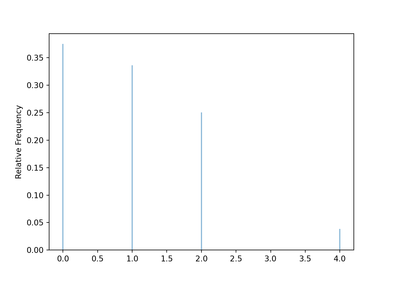

Now we can easily investigate different values of $n$ . For example, for $n=10$ we see that the probability of at least one match is around 0.63 and the long run average number of matches is around 1.


matching_sim(10)

## (0.6277, 0.9965)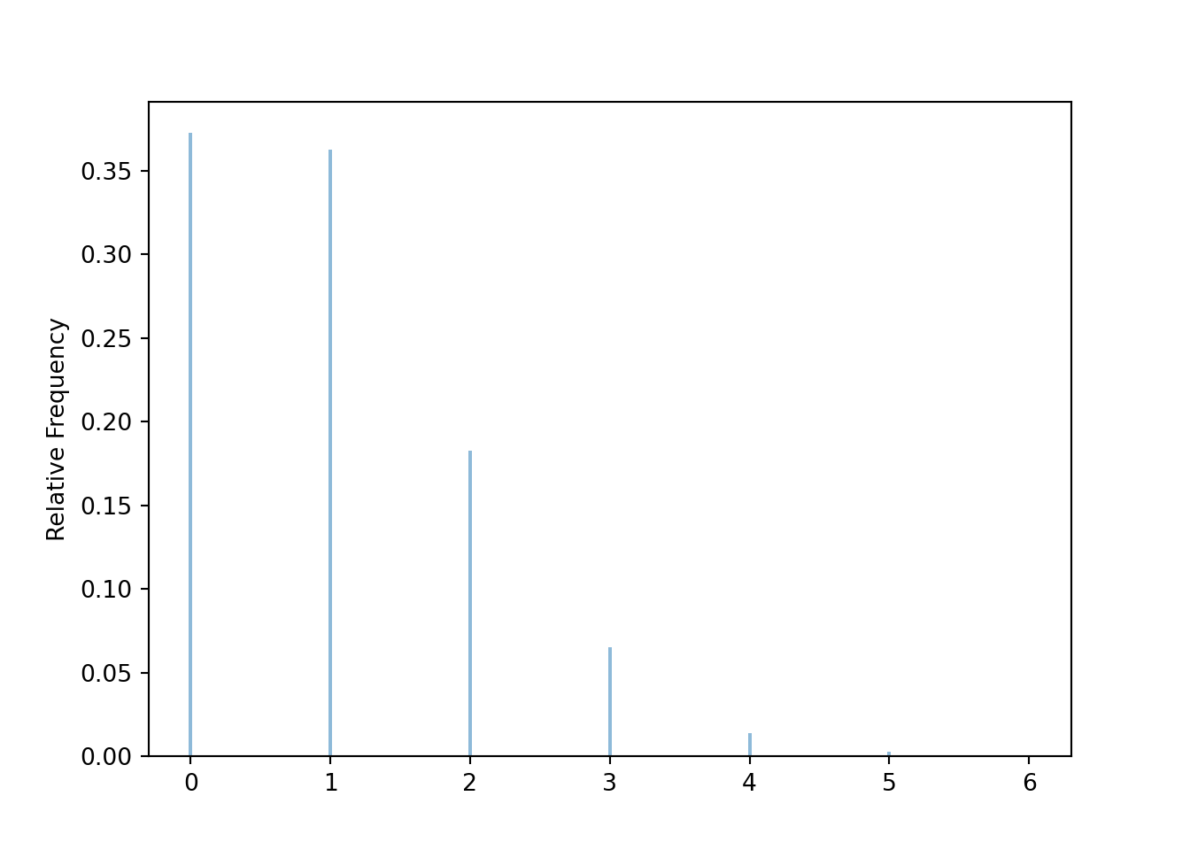

We can use a for loop to automate the process of changing the value of $n$ , running the simulation, and recording the results. If ns is the list of $n$ values of interest we basically just need to run

for n in ns:
    matching_sim(n)

In Python we can also use list comprehension

[matching_sim(n) for n in ns]

The table below summarizes the simulation results for $n=4, \ldots, 10$ . The first line defines the values of $n$ , and the second line implements the for loop. The tabulate code just adds a little formatting to the table. Note that we have temporarily redefined matching_sim to remove the lines that produced the plot, but we have not displayed the revised code here. (We will get bring the plot back soon.)


ns = list(range(4, 11, 1))

results = [matching_sim(n) for n in ns]

print(tabulate({'n': ns,
                'P(Y > 0), LRA': results},
               headers = 'keys', floatfmt=".3f"))

##   n  P(Y > 0), LRA
## ---  ----------------
##   4  (0.6229, 0.9962)
##   5  (0.6298, 0.9806)
##   6  (0.6316, 1.0037)
##   7  (0.634, 1.0025)
##   8  (0.6333, 0.9979)
##   9  (0.6261, 0.9824)
##  10  (0.631, 0.9932)

Stop and look at the table; what do you notice? How do the probability of at least one match and the long run average value depend on $n$ ? They don’t! Well, maybe they do, but they don’t appear to change very much with $n$ after we take into account simulation margin of error⁸⁶ of about 0.01-0.02. It appears that regardless of the value of $n$ , the probability of at least one match is around 0.63 and the long run average number of matches is around 1.

If we’re interested in more values of $n$ , we just repeat the same process with a longer list of ns. The code below uses Matplotlib to create a plot of the probability of at least one match and the long run average number of matches versus $n$ . While there is some natural simulation variability, we see that the probability of at least one match (about 0.63) and the long run average value (about 1) basically do not depend on $n$ !


ns = list(range(4, 101, 1))

results = [matching_sim(n) for n in ns]

plt.figure()
plt.plot(ns, results)
plt.legend(['P(Y > 0)', 'LRA'])
plt.xlabel('n')
plt.ylabel('value')
plt.show()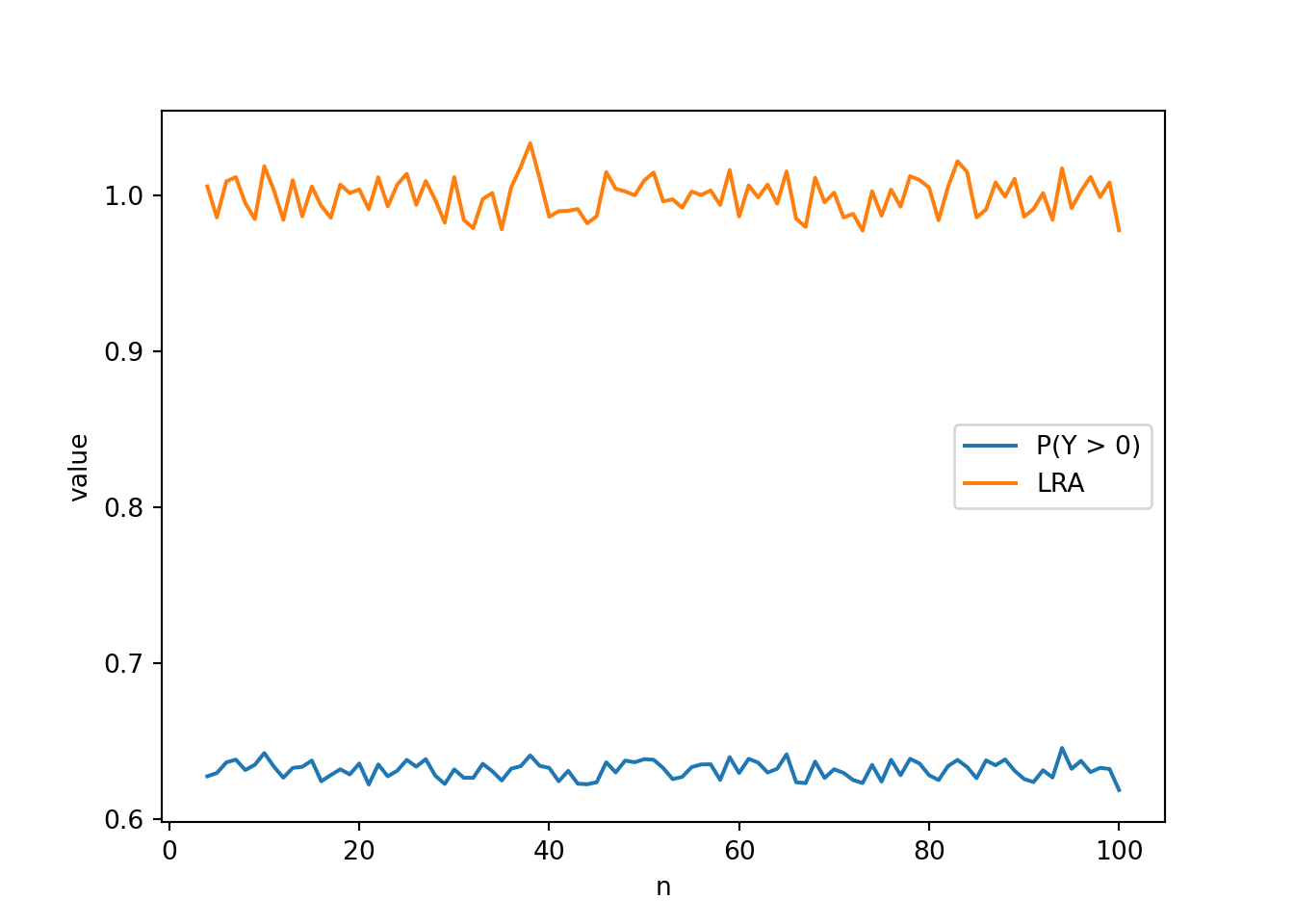

What about the distribution of $Y$ ? Clicking on the picture below will launch a Colab notebook that contains code for investigating how the distribution of $Y$ depends on $n$ . The basic simulation code is identical to what we have already seen. The notebook adds a few lines to create a Jupyter widget, which produces an interactive plot (with some additional formatting) of the distribution with a slider; you can change the slider to see how the distribution of $Y$ changes with $n$ . Take a few minutes to play with the slider; what do you see?

Sorry, something went wrong. Reload?

Sorry, we cannot display this file.

Sorry, this file is invalid so it cannot be displayed.

view raw matching-problem-simulation.ipynb hosted with ❤ by GitHub

You should see that unless $n$ is really small (like 4 or 5) the distribution of $Y$ is basically the same for any value of $n$ ! And the distribution appears to follow a distribution called the Poisson(1) distribution. In particular, the probability of exactly 0 matches is approximately equal to the probability of exactly 1 match.

Summarizing, our simulation investigation of the matching problem reveals that, unless $n$ is really small,

the probability of at least one match does not depend on $n$ , and is approximately 0.632.
the long run average number of matches is approximately 1
the distribution of the number of matches is approximately the same for all values of $n$
the distribution of the number of matches is approximately the Poisson(1) distribution.

We will investigate these observations further later. For now, marvel at the fact that no matter if there are 10 or 10 thousand or 10 million rocks and spots, there is about a 63% probability that at least one rock will be in the correct spot. Amazing!

2.14.1 Summary

We can use Python code to
- define functions to define random variables
- define for loops to investigate changing parameters
- customize plots produced by the Symbulate plot command (add axis labels, legends, etc)
- summarize results of multiple simulations in tables and Matplotlib plots (e.g., for different values of problem parameters)
Simulation provides an effective way for investigation probability problems
Probability problems can have surprising results!

The simulation margin of error for a single probability of at least one match is about 0.01 based on 10000 simulated values. We haven’t discussed simulation margins of error for long run averages yet. In this case, the simulation margin of error for a single long run average based on 10000 simulated values is about 0.02.↩︎