3.7 Uniform probability measures

For a finite sample space with equally likely outcomes, computing the probability of an event reduces to counting the number of outcomes that satisfy the event. The continuous analog of equally likely outcomes is a uniform probability measure. When the sample space is uncountable, size is measured continuously (length, area, volume) rather that discretely (counting).

\[ \textrm{P}(A) = \frac{|A|}{|\Omega|} = \frac{\text{size of } A}{\text{size of } \Omega} \qquad \text{if $\textrm{P}$ is a uniform probability measure} \]

Example 3.29 In the meeting problem, assume that Regina arrives at a time chosen uniformly at random between noon and 1. If we measure measure time in minutes after noon, we can model Regina’s arrival with the sample space $[0, 60]$ and a uniform probability measure.

Find the probability that Regina arrives before 12:15.
Find the probability that Regina arrives after 12:45.
Find the probability that Regina arrives between 12:15 and 12:45.
Find the probability that Regina arrives between 12:15:00 and 12:16:00.
Find the probability that Regina arrives between 12:15:00 and 12:15:01.
Find the probability that Regina arrives at the exact time 12:15:00 (with infinite precision).

Solution. to Example 3.29

Show/hide solution

Since the sample space is $[0, 60]$, a continuous (one-dimensional) interval, “size” is measured by length (which in this context represents fractions of an hour). Let $\textrm{P}$ be the uniform probability measure on $[0, 60]$. The interval from noon to 12:15 has length 15 minutes and the sample space has length 60 minutes, so the probability she arrives before 12:15 is $15/60 = 0.25$; $\textrm{P}([0, 15)) = 0.25$.
Similar to the previous part, the probability she arrives after 12:45 is 0.25; $\textrm{P}((45, 60]) = 0.25$.
The probability that Regina arrives between 12:15 and 12:45, an interval of length 30 minutes, is 30/60 = 0.5; $\textrm{P}((15, 45)) = 0.5$.
A one minute interval has probability $1/60$, so the probability she arrives between 12:15 and 12:16 is 0.0167; $\textrm{P}([15, 15+1]) = 1/60$.
A one second interval has length 1/60 and probability (1/60)/60 = 1/3600, so the probability she arrives between 12:15:00 and 12:15:01 is 0.000278; $\textrm{P}([15, 15+1/60]) = 1/3600$.
The exact time 12:15:00 represents a single point the sample space, an interval of length 0. The probability that Regina arrives at the exact time 12:15:00 (with infinite precision) is 0; $\textrm{P}(\{15\}) = 0$.

The last part in the previous example might seem counterintuitive at first, but we have already seen similar ideas in simulations. There was nothing special about 12:15; pick any time in the continuous interval from noon to 1:00, and the probability that Regina arrives at that exact time, with infinite precision, is 0. This idea can be understood as a limit. The probability that Regina arrives within one minute of the specified time is small, within one second of the specified time is even smaller, within one millisecond of the specified time is even smaller still; with infinite precision these time increments can get smaller and smaller indefinitely. Of course, infinite precision is not practical, but assuming the possible arrival times are represented by a continuous interval provides a reasonable mathematical model. Even though any particular time has probability 0 of being the exact arrival time, intervals of time still have positive probability of containing the arrival time. This is one reason why probabilities are defined for events and not outcomes.

For a continuous sample space, the probability of any particular outcome is 0. For a continuous random variable, the probability it takes any particular value is 0.

The sample space in the previous problem was one-dimensional, and size was measured with length. Example 2.24 involves a uniform probability measure for a two-dimensional sample space where size is measured by area. The following is another two-dimensional example.

Example 3.30 Katniss throws a dart at a circular dartboard with radius 1 foot. Suppose that Katniss’s dart lands at a uniformly random location on the dartboard (and she never misses the dartboard).

Compute the probability that Katniss’s dart lands within 1 inch of the center of the dartboard.
Compute the probability that Katniss’s dart lands more than 1 inch but less than 2 inches away from the center of the dartboard.
Compute the probability that Katniss’s dart lands within 1 inch of the outside edge of the dartboard (but on the dartboard).
Continue the previous parts for the remaining 1 inch increments from the center to the edge of the dartboard.
Let $R$ be the distance (inches) from the location of the dart to the center of the dartboard. Find $\textrm{P}(R < 1)$.
Find $\textrm{P}(1 < R < 2)$.
Sketch a plot of the distribution of $R$. Does $R$ follow a Uniform distribution?
Find and interpret the 50th percentile of $R$.
Find and interpret the 25th percentile of $R$.
Find and interpret the 75th percentile of $R$.
Sketch a spinner corresponding to the distribution of $R$.

Solution. to Example 3.30

Show/hide solution

The area of the whole board is $\pi$ (sqft), which account for 100% of the probability. Within 1 inch of center corresponds to an area of $(1/12)^2\pi$ sqft. So since the location is Uniform, the probability is $\frac{(1/12)^2\pi}{\pi}=(1/12)^2 = 0.00694$.
The probability that it lands within 2 inches of center is $\frac{(2/12)^2\pi}{\pi} = (2/12)^2$. So the probability that it lands more than 1 inch but less than 2 inches of center is $\frac{(2/12)^2\pi - (1/12)^2\pi}{\pi} = (2/12)^2 - (1/12)^2 = 0.0208$
Area of region of interest is $\pi - (11/12)^2\pi$, so the probability is $\frac{\pi - (11/12)^2\pi}{\pi} = 1-(11/12)^2 = 0.1597$.
Continuing in the previous manner, the probability that the dart is between $x$ and $x-1$ inches away from center is $(x/12)^2-((x-1)/12)^2$.
Since $R<1$ if and only if the dart is within 1 inch of center, this follows from part 1: $\textrm{P}(R<1) = (1/12)^2$.
This follows from part 2: $\textrm{P}(1<R<2) = (2/12)^2 - (1/12)^2$.
$R$ takes values in [0, 12], but $R$ is more likely to be close to 12 than to 0, so $R$ does not follow a uniform distribution. Split the interval from [0, 12] inches into 1 inch bins and use the previous parts to construct a histogram. For example, the bin for [0, 1] inch will have area 0.00694 and the bin for [11, 12] inches will have area 0.1597. See Figure 3.5.
For $0<r<12$, $R< r$ if the dart lands within $r$ inches of center. So $\textrm{P}(R < r) = (r/12)^2\pi/\pi = (r/12)^2$. The 50th percentile satisfies $\textrm{P}(R < r) = 0.5$, so set $(r/12)^2=0.5$ and solve to find the 50th percentile is $12\sqrt{0.5} = 8.49$ inches. Half of Katniss’s throws will be more than 8.49 inches away from center, and half less. It is equally likely that the throw will be more or less than 8.49 inches from center.
The 25th percentile satisfies $\textrm{P}(R < r) = 0.25$, so set $(r/12)^2=0.25$ and solve to find the 25th percentile is $12\sqrt{0.25} = 6$ inches. 25% of Katniss’s throws will be less than 6 inches away from center, and 75% more than 6 inches. It is 3 times more likely that the throw will be more than 6 inches away from center than less than 6 inches away from center.
The 75th percentile satisfies $\textrm{P}(R < r) = 0.75$, so set $(r/12)^2=0.75$ and solve to find the 75th percentile is $12\sqrt{0.75} = 10.39$ inches. 75% of Katniss’s throws will be less than 10.39 inches away from center, and 25% more than 10.39 inches. It is 3 times more likely that the throw will be less than 10.39 inches away from center than more than 10.39 inches away from center.
See Figure 3.6. The 25th, 50th, 75th percentiles go at “3, 6, 9 o’clock” respectively. We have filled in a few more percentiles using a method similar to the previous parts. Note that the values on the circular axis are not evenly spaced.

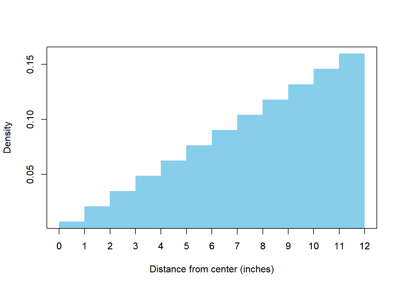
$Histogram representing the marginal distribution of $R$ in Example 3.30.$

Figure 3.5: Histogram representing the marginal distribution of $R$ in Example 3.30.

$Spinner representing the marginal distribution of $R$ in Example 3.30.$

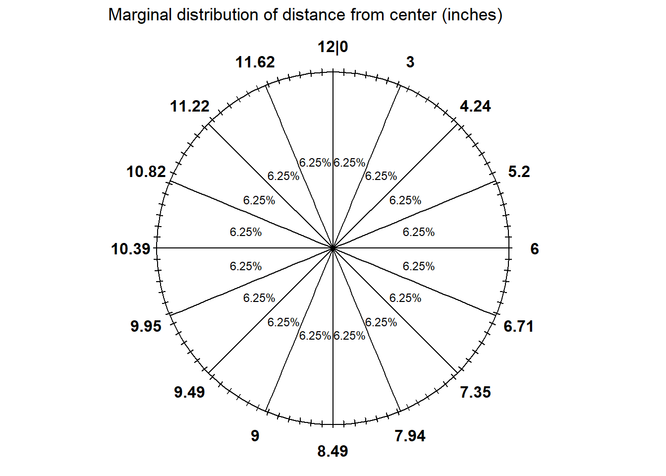
Figure 3.6: Spinner representing the marginal distribution of $R$ in Example 3.30.

In the previous problem we see that even though the dart hits the board at a uniformly randomly location, its distance from the center does not follow a uniform distribution. Let’s look at a simulation. It’s a little tricky to simulate a point at random in a circle, but here’s onle way. Assume that the center of the dartboard is at (0, 0) so that each of the $(x, y)$ coordinates of the location of the dart is between $-1$ and 1. We can simulate $X$ and $Y$ coordinates independently each from a Uniform(-, 1) distribution.

X, Y = RV(Uniform(-1, 1) ** 2)

(X & Y).sim(1000).plot()

Unfortunately, this simulates points at random in the square with sides $[-1, 1]$ and results in darts off the board. Therefore, we want to discard any $(X, Y)$ points for which $R = sqrt{X^2 + Y^2$, }the distance to the center (0, 0), is greater than 1. We can do this with conditioning.

R = sqrt(X ** 2 + Y ** 2)

x_and_y = ( (X & Y) | (R < 1) ).sim(10000)

x_and_y.plot()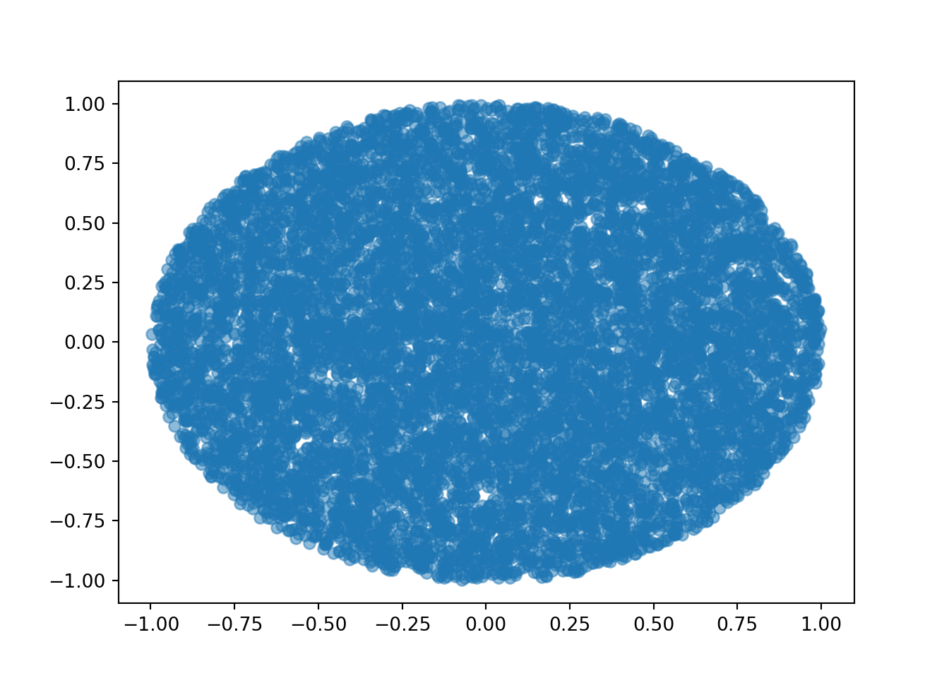

The $(X, Y)$ pairs appear to be uniformly distributed over the unit circle. Now we summarize the approximate marginal distribution of $R$.

x = x_and_y[0]
y = x_and_y[1]

r = 12 * sqrt(x ** 2 + y ** 2) # "12 *" to convert distance from feet to inches

r.plot(bins = 12)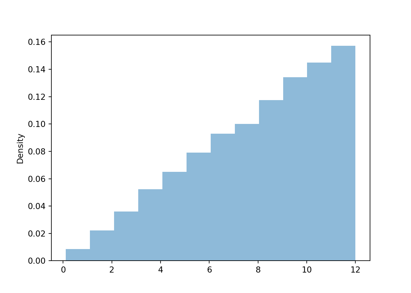

The simulation-based approximations agree with our calculations.

r.count_lt(1) / r.count()

## 0.0074

r.count_gt(11) / r.count()

## 0.1567

r.quantile(0.25)

## 5.937908719549644

[r.quantile(p) for p in [0.25, 0.5, 0.75]]

## [5.937908719549644, 8.480404351832334, 10.382042982415898]

Here are the other percentiles that are displayed on the spinner.

increments = range(1, 16)

percentile = [i / 16 for i in increments]

percentile_value = [r.quantile(p) for p in percentile]

print(tabulate({'Percentile': percentile,
                'Value': percentile_value},
               headers = 'keys', floatfmt=".4f"))

##   Percentile    Value
## ------------  -------
##       0.0625   2.9998
##       0.1250   4.2088
##       0.1875   5.1538
##       0.2500   5.9379
##       0.3125   6.6323
##       0.3750   7.2879
##       0.4375   7.8992
##       0.5000   8.4804
##       0.5625   8.9782
##       0.6250   9.4915
##       0.6875   9.9260
##       0.7500  10.3820
##       0.8125  10.8079
##       0.8750  11.2099
##       0.9375  11.6140

3.7.1 Non-uniform probability measures

Most random phenomenon do not involve equally likely outcomes or uniform probability measures. Even when the underlying outcomes are equally likely, the values of related random variables are usually not. Therefore, most interesting probability problems involve non-uniform probability measures.

For countable sample spaces, a probability measure is often defined by specifying the probability of each individual outcome. The probability of any event can then be obtained (using countable additivity) by summing the probabilities of the outcomes which comprise the event. Such was the case in Example 2.22. We specified the relative likelihood of each outcome, and then we obtained probabilities of all the events in Table 2.10 by adding the appropriate outcome probabilities. For example, the probability that the result of a single roll of the die in Example 2.22 results in an even number is $\tilde{\textrm{Q}}(\{2, 4\}) = \tilde{\textrm{Q}}(\{2\}) + \tilde{\textrm{Q}}(\{4\}) = 6/15 + 2/15 = 8/15$.

For uncountable sample spaces, specifying probabilities for individual outcomes is not a feasible strategy. As illustrated by Example 3.29 and the discussion following it, reasonable mathematical models for outcomes taking values on a continuous scale, with infinite precision, assign 0 probability to any exact outcome. Therefore, we specify a probability measure for uncountable sample spaces by assigning probabilities to intervals or regions of the sample space.

Example 3.31 In the meeting problem we’ll consider only Regina’s arrival time again. We will model Regina’s arrival time with the sample space $[0, 60]$ and a non-uniform probability measure which reflects that she is more likely to arrive closer to 1 than to noon. In particular, we assume that the probability that Regina arrives before time $x\in [0, 60]$ is equal to $(x/60)^2$; let $\textrm{Q}$ denote the corresponding probability measure. (We will see where such a probability measure might come from later. For now, we’ll just use it to compute probabilities and observe that it is a non-uniform measure.) In addition to computing probabilities below, compare your answers to the corresponding parts from Example 3.29.

Find the probability that Regina arrives before 12:15.
Find the probability that Regina arrives after 12:45. How does this compare to the previous part? What does that say about Regina’s arrival time?
Find the probability that Regina arrives between 12:15 and 12:45.
Find the probability that Regina arrives between 12:15:00 and 12:16:00.
Find the probability that Regina arrives between 12:15:00 and 12:15:01.
Find the probability that Regina arrives at the exact time 12:15:00 (with infinite precision).
Find the probability that Regina arrives between 12:59:00 and 1:00:00. How does this compare to the probability for 12:15:00 to 12:16:00? What does that say about Regina’s arrival time?
Find the probability that Regina arrives between 12:59:59 and 1:00:00. How does this compare to the probability for 12:15:00 to 12:15:01? What does that say about Regina’s arrival time?
Find the probability that Regina arrives at the exact time 1:00:00 (with infinite precision).

Solution. to Example 3.31

Show/hide solution

Notice that $\textrm{Q}([0, 60]) = (60/60)^2 = 1$, so $\textrm{Q}$ is a valid probability measure. 12:15 corresponds to arriving at time $15$, so by assumption the probability she arrives before 12:15 is $(15/60)^2 =0.25^2 0.0625$; $\textrm{Q}([0, 15)) = 0.0625$. (She is now less likely to arrive within 15 minutes of noon than in the uniform case.)
12:45 corresponds to arriving at time 45 and by assumption the probability she arrives before 12:45 is $(45/60)^2 = 0.75^2 =0.5625$. Therefore, the probability that she arrives after 12:45, i.e., in the interval $[45, 60]$ is $\textrm{Q}([45, 60]) = 1 - 0.5625 = 0.4375$. So she is 7 times more likely to arrive within 15 minutes of 1:00 than within 15 minutes of noon. (She is now more likely to arrive with 15 minutes of 1:00 than in the uniform case.)
The probability that Regina arrives between 12:15 and 12:45 is $\textrm{Q}((15, 0.45)) = 1 - 0.0625 - 0.4375 = 0.5$. (This probability happens to be the same as in the uniform case.)
The probability that she arrives before 12:16 is the sum of the probability that she arrives before 12:15 and the probability that she arrives between 12:15 and 12:16. Therefore, \[\begin{align*} \textrm{Q}([15, 15 + 1]) & = \textrm{Q}([0, 15 + 1]) - \textrm{Q}([0, 15])\\ & = (0.25 + 1/60)^2 - 0.25^2 = 0.0086. \end{align*}\] (This probability is less than what it was in the uniform case.)
Similar to the previous part, $\textrm{Q}([15, 15+1/60]) = (0.25 + 1/3600)^2 - 0.25^2 = 0.00014$. (This probability is less than what it was in the uniform case.)
The exact time 12:15:00 represents a single point the sample space, an interval of length 0. The probability that Regina arrives at the exact time 12:15:00 (with infinite precision) is 0; $\textrm{Q}(\{15\}) = 0$.
$\textrm{Q}([60 - 1, 1]) = \textrm{Q}([0, 60]) - \textrm{Q}([0, 60 - 1]) = 1^2 - (1-1/60)^2 = 0.0331$. Notice that this one minute interval around 1:00 has higher probability that a one minute interval around 12:15. (This probability is more than what it was in the uniform case.)
Similar to the previous part, $\textrm{Q}([1-1/60, 1]) = 1^2 - (1-1/3600)^2 = 0.00056$. Notice that this one second interval around 1:00 has higher probability that a one second interval around 12:15, though both probabilities are small. (This probability is more than what it was in the uniform case.)
The exact time 1:00:00 represents a single point the sample space, an interval of length 0. The probability that Regina arrives at the exact time 1:00:00 (with infinite precision) is 0; $\textrm{Q}(\{60\}) = 0$.

In Example 3.31, the probability that Regina arrives at any exact time in $[0, 60]$, with infinite precision, is 0, just as in Example 3.29. But the values of the probabilities in Example 3.31 illustrate the non-uniform probability assumption. Regina is much more likely to arrive between 12:45 and 1:00 than she is to arrive between 12:00 and 12:15, even though both these intervals have the same length. Also, while the probability that she arrives at any exact time with infinite precision is 0, the probability that she arrives “close to” 1:00 is larger than the probability that she arrives “close to” 12:15 (where “close to” might mean within a minute or within a second.) See Figure 3.7 which displays Regina’s probability of arriving at each minute, rounded to the nearest minute, under both the uniform and non-uniform probability measures. In some sense, some values in $[0, 60]$ are “more likely” than others under the non-uniform measure. We will explore this idea further later, where we will see that integration plays the analogous role for uncountable sample spaces that summation plays for countable sample spaces.

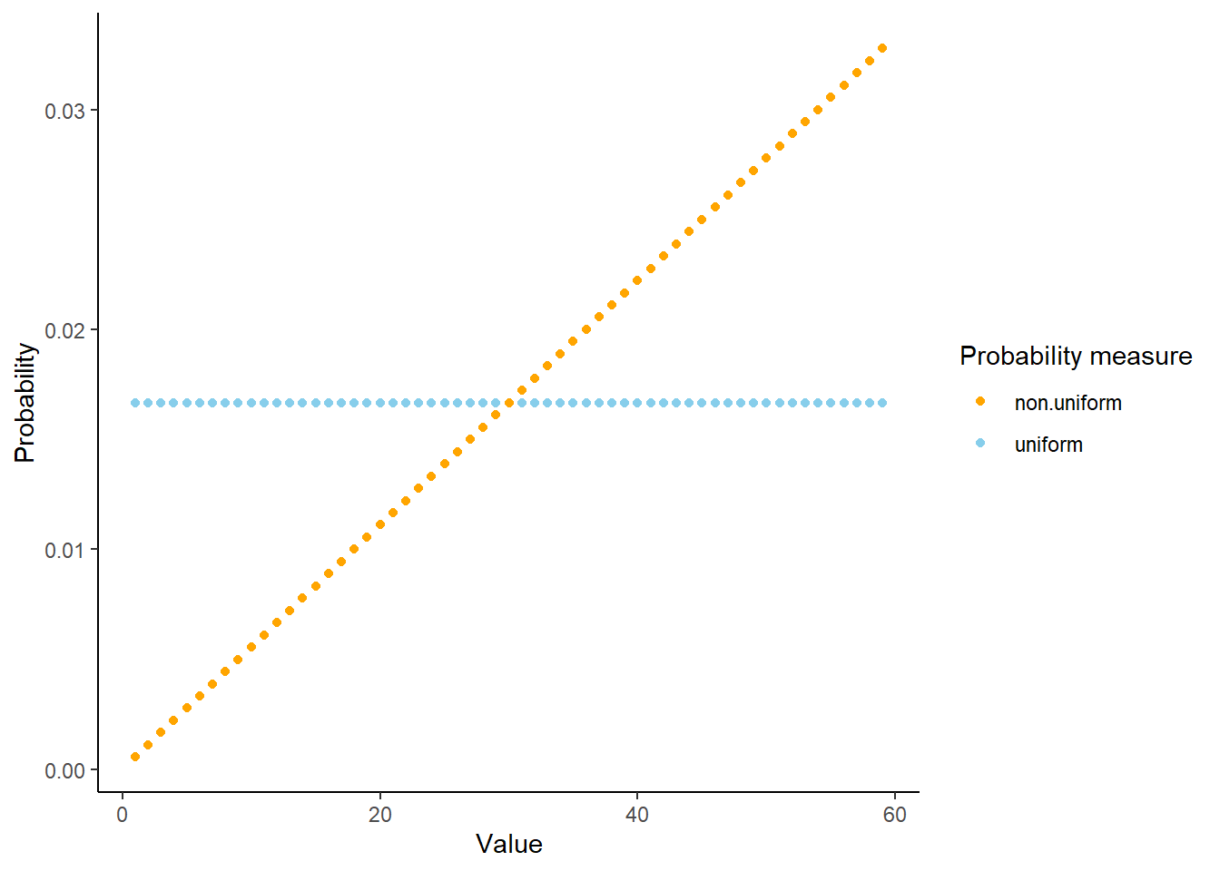
Probability of Regina arriving at each minute between noon (0) and 1:00PM (60), to the nearest minute, for the Uniform probability measure (blue) and the probability measure in Example 3.31 (orange).

Figure 3.7: Probability of Regina arriving at each minute between noon (0) and 1:00PM (60), to the nearest minute, for the Uniform probability measure (blue) and the probability measure in Example 3.31 (orange).