3.2 Law of total probability
The law of total probability says that a marginal probability can be thought of as a weighted average of “case-by-case” conditional probabilities, where the weights are determined by the likelihood of each case.
Example 3.3 Each question on a multiple choice test has four options. You know with certainty the correct answers to 70% of the questions. For 20% of the questions, you can eliminate two of the incorrect choices with certainty, but you guess at random among the remaining two options. For the remaining 10% of questions, you have no idea and guess one of the four options at random.
Randomly select a question from this test. What is the probability that you answer the question correctly?
- Construct an appropriate twoway table and use it to find the probability of interest.
- For any given question on the exam, your probability of answering it correctly is either 1, 0.5, or 0.25, depending on if you know it, can eliminate two choices, or are just guessing. How does your probability of correcting answering a randomly selected question relate to these three values? Which value — 1, 0.5, or 0.25 —is the overall probability closest to, and why?
Solution. to Example 3.3
Show/hide solution
Suppose there are 1000 questions on the test. (That’s a long test! But remember, 1000 is just a convenient round number.) We can classify each question by its type (know, eliminate, guess) and whether we answer it correctly or not. The probability that we answer a question correctly is 1 given that we know it, 0.5 given that we can eliminate two choices, or 0.25 given that we guess randomly.
Know Eliminate Guess Total Correct 700 100 25 825 Incorrect 0 100 75 175 Total 700 200 100 1000 The probability that we answer a randomly selected question correctly is 825/1000 = 0.825.
The overall probability of answering a question correctly is closer to 1 than 0.5 or 0.25. To construct the table and obtain the value 0.825, we basically did the following calculation
\[ 0.825 = (1)(0.7) + (0.5)(0.2) + (0.25)(0.1) \]
We see that the overall probability, 0.825, is a weighted average of the case-by-case probabilities 1, 0.5, and 0.25, where 1 gets the most weight in the average because there is a higher percentage of questions that we know.
Law of total probability. If \(C_1,\ldots, C_k\) are disjoint with \(C_1\cup \cdots \cup C_k=\Omega\), then \[\begin{align*} \textrm{P}(A) & = \sum_{i=1}^k \textrm{P}(A \cap C_i)\\ & = \sum_{i=1}^k \textrm{P}(A|C_i) \textrm{P}(C_i) \end{align*}\]
The events \(C_1, \ldots, C_k\), which represent the “cases”, form a partition of the sample space; each outcome \(\omega\in\Omega\) lies in exactly one of the \(C_i\). The law of total probability says that we can interpret the unconditional probability \(\textrm{P}(A)\) as a probability-weighted average of the case-by-case conditional probabilities \(\textrm{P}(A|C_i)\) where the weights \(\textrm{P}(C_i)\) represent the probability of encountering each case.
For an illustration of the law of total probability, consider the mosaic plot in in Figure 3.2. The heights of the bars for each type correspond to the conditional probabilities of answering correctly given type (1, 0.5, 0.25). The widths of these bars are scaled in proportion to the marginal probability of type; the width of the bar for the “know” type is 7 times wider than the width for the “guess” type. The single bar to the right displays the marginal probability of answering a question correctly or not. The height within this marginal bar (0.825) is the weighted average of the heights within the other bars (the conditional probabilities of correct given type), with the weights given by the widths of the other bars (the marginal probabilities of type).
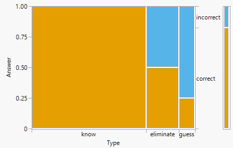
Figure 3.2: (ref:cap-ltp-multiple-choice)
Example 3.4 Imagine a light that flashes every few seconds90. The light randomly flashes green with probability 0.75 and red with probability 0.25, independently from flash to flash.
- Write down a sequence of G’s (for green) and R’s (for red) to predict the colors for the next 40 flashes of this light. Before you read on, please take a minute to think about how you would generate such a sequence yourself.
- Most people produce a sequence that has 30 G’s and 10 R’s, or close to those proportions, because they are trying to generate a sequence for which each outcome has a 75% chance for G and a 25% chance for R. That is, they use a strategy in which they predict G with probability 0.75, and R with probability 0.25. How well does this strategy do? Compute the probability of correctly predicting any single item in the sequence using this strategy.
- Describe a better strategy. (Hint: can you find a strategy for which the probability of correctly predicting any single flash is 0.75?)
Solution. to Example 3.4
Show/hide solution
- As mentioned above, most people produce a sequence that has 30 G’s and 10 R’s, or close to those proportions, because they are trying to generate a sequence for which each outcome has a 75% chance for G and a 25% chance for R. That is, they use a strategy in which they predict G with probability 0.75, and R with probability 0.25.
- There are two cases: the true flash is either green (with probability 0.75) or red (with probability 0.25). Given that the flash is green, your probability of correctly predicting it is 0.75 (because your probability of guessing “G” is 0.75). Given that the flash is red, your probability of correctly predicting it is 0.25 (because your probability of guessing “R” is 0.25). Use the law of total probability to find the probability that your prediction is correct: \((0.75)(0.75) + (0.25)(0.25) = 0.625\).
- Just pick G every time! Picking green every time has a 0.75 probability of correctly predicting any flash. When events are independent, trying to guess the pattern doesn’t help.
Conditioning and using the law of probability is an effective strategy in solving many problems, even when the problem doesn’t seem to involve conditioning. For example, when a problem involves iterations or steps it is often useful to condition on the result of the first step.
Example 3.5 You and your friend are playing the “lookaway challenge”.
The game consists of possibly multiple rounds. In the first round, you point in one of four directions: up, down, left or right. At the exact same time, your friend also looks in one of those four directions. If your friend looks in the same direction you’re pointing, you win! Otherwise, you switch roles and the game continues to the next round — now your friend points in a direction and you try to look away. As long as no one wins, you keep switching off who points and who looks. The game ends, and the current “pointer” wins, whenever the “looker” looks in the same direction as the pointer.
Suppose that each player is equally likely to point/look in each of the four directions, independently from round to round. What is the probability that you win the game?
- Why might you expect the probability to not be equal to 0.5?
- If you start as the pointer, what is the probability that you win in the first round?
- If \(p\) denotes the probability that the player who starts as the pointer wins the game, what is the probability that the player who starts as the looker wins the game? (Note: \(p\) is the probability that the person who starts as pointer wins the whole game, not just the first round.)
- Condition on the result of the first round and set up an equation to solve for \(p\).
- How much more likely is the player who starts as the pointer to win than the player who starts as the looker?
Solution. to Example 3.5
Show/hide solution
- The player who starts as the pointer has the advantage of going first; that player can win the game in the first round, but cannot lose the game in the first round. So we might expect the player who starts as the pointer to be more likely to win than the player who starts as the looker.
- 1/4. If we represent an outcome in the first round as a pair (point, look) then there are 16 possible equally likely outcomes, of which 4 represent pointing and looking in the same direction. Alternatively, whichever direction the pointer points, the probability that the looker looks in the same direction is 1/4.
- \(1-p\), since the game keeps going until someone wins.
- Here is where we use conditioning and the law of total probability. We condition on what happens in the first round: either the person who starts as the pointer wins the first round and the game ends (event \(B\)), or the person who starts as the pointer does not win the the first round and the game continues with the other player becoming the pointer for the next round (event \(B^c\)). Let \(A\) be the event that the person who starts as the pointer wins the game, and \(B\) be the event that the person who starts as the pointer wins in the first round. By the law of total probability \[ \textrm{P}(A) = \textrm{P}(A|B)\textrm{P}(B) + \textrm{P}(A|B^c)\textrm{P}(B^c) \] Now \(\textrm{P}(A)=p\), \(\textrm{P}(B)=1/4\), \(\textrm{P}(B^c)=3/4\), and \(\textrm{P}(A|B)=1\) since if the person who starts as the pointer wins the first round then they win the game. Now consider \(\textrm{P}(A|B^c)\). The key is to recognize that if the person who starts as the pointer does not win in the first round, it is like the game starts over with the other playing starting as the pointer. That is, the player who originally started as the pointer, having not won the first round, is now starting as the looker, and the probability that the player who starts as the looker wins the game is \(1-p\). That is, \(\textrm{P}(A|B^c) = 1-p\). Therefore \[ p = (1)(1/4)+ (1-p)(3/4) \] Solve to find \(p=4/7\approx 0.57\).
- The player who starts as the pointer is about \((4/7)/(3/7) = 4/3\approx 1.33\) times more likely to win the game than the player who starts as the looker.
The following is one way to code the lookaway challenge. In each round an outcome is a (point, look) pair, coded with a BoxModel with size=2 (and choices labeled 1, 2, 3, 4). The ** inf assumes the rounds continue indefinitely, so the outcome of a game is a sequence of (point, look) pairs for each round. The random variable \(X\) counts the number of rounds until there is a winner, which occurs in the first round that point = look. The player who goes first wins the game if the game ends in an odd number of rounds, so to estimate the probability that the player who goes first wins we find the proportion of repetitions in which \(X\) is an odd number.
def is_odd(x):
    return (x % 2) == 1

def count_rounds(sequence):
    for r, pair in enumerate(sequence):
        if pair[0] == pair[1]:
            return r + 1 # +1 for 0 indexing

P = BoxModel([1, 2, 3, 4], size = 2) ** inf

X = RV(P, count_rounds)

x = X.sim(10000)
x.plot()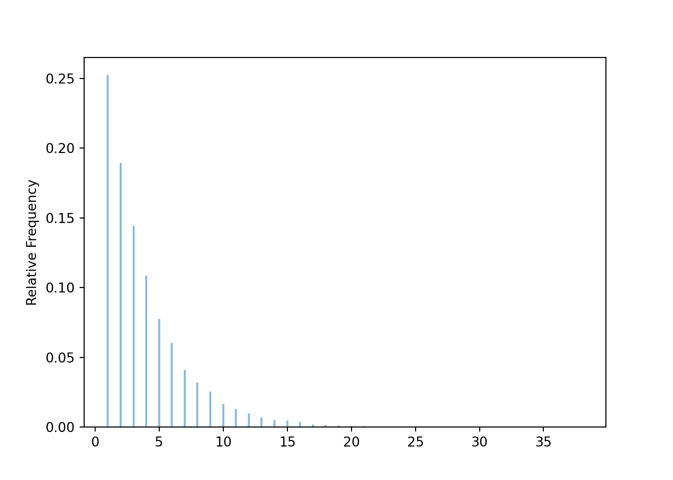
x.count(is_odd) / x.count()## 0.5699The simulation coded the individual rounds. However, the law of total probability allowed us to take advantage of the iterative nature of the game, and consider only one round rather than enumerating all the possibilities of what might happen over many potential rounds.
Thanks to Allan Rossman for this example.↩︎