2.7 Conditioning
Conditioning concerns how probabilities of events or distributions of random variables are influenced by information about the occurrence of events or the values of random variables. (Later, we will also see that conditioning provides a useful strategy for breaking problems down into smaller parts.)
A probability is a measure of the likelihood or degree of uncertainty of an event. A conditional probability revises this measure to reflect any “new” information about the outcome of the underlying random phenomenon.
Example 2.32 The probability66 that a randomly selected American adult supports impeachment of President Trump is 0.49.
- Suppose the randomly selected person is a Democrat. Do you think the probability that the randomly selected Democrat supports impeachment is 0.49?
- The probability67 that a randomly selected American is a Democrat is 0.31. Donny Don’t68 says that the probability that a randomly selected American both (1) is a Democrat, and (2) supports impeachment is equal to \(0.49\times 0.31\). Do you agree?
- Without further information, provide a range of “logically possible” values for the probability in the previous part. (“Logically possible” means they satisfy the rules of probability, even though they might not be realistic in context.)
- Suppose that the probability that a randomly selected American both is a Democrat and supports impeachment is 0.26. Construct an appropriate two-way table of probabilities.
- Construct a corresponding two-way table of hypothetical counts.
- Find the probability69 that a randomly selected American who is a Democrat supports impeachment.
- How can the probability in the previous part be written in terms of the probabilities provided in the setup?
- Find the probability that a randomly selected American who supports impeachment is a Democrat.
Solution. to Example 2.32
Show/hide solution
The probability that the randomly selected Democrat supports impeachment is probably a lot larger than 0.49. Knowing that the selected person is a Democrat would change the probability of supporting impeachment.
No. Consider a hypothetical set of 100 Americans. We would expect about 31 of these 100 Americans to be Democrats. However, we would not expect just 15 — that is, about half (\((0.49)(31)\approx 15\)) — of the 31 Democrats to support impeachment; we’d expect more, say 26 out of the 31. If 26 of the 100 Americans are Democrats who support impeachment, this would be consistent with a value of 0.26 for the probability that a randomly selected American both (1) is a Democrat, and (2) supports impeachment equal.
We could make a table like in the following part and see what values produce valid tables. If \(A\) is the event that the selected person supports impeachment, and \(D\) is the event that the person is a Democrat, and \(\textrm{P}\) corresponds to randomly selecting an American, then \(\textrm{P}(A) = 0.49\) and \(\textrm{P}(D) = 0.31\). By the subset rule \(\textrm{P}(A\cap B)\le \min(\textrm{P}(A), \textrm{P}(D)) = 0.31\). The largest \(\textrm{P}(A\cap D)\) can be is 0.31, which corresponds to all Democrats supporting impeachment. In this case, the smallest \(\textrm{P}(A \cap D)\) can be is 0, which corresponds to no Democrats supporting impeachment. The extremes are not realistic, but without knowing more information, we do not know where \(\textrm{P}(A\cap D)\) lies in \(0\le \textrm{P}(A \cap D) \le 0.31\).
If the probability that a randomly selected American both is a Democrat and supports impeachment is 0.26, then the two-way table of probabilities is
\(A\) \(A^c\) Total \(D\) 0.26 0.05 0.31 \(D^c\) 0.23 0.46 0.69 Total 0.49 0.51 1.00 It is often much easier to work with counts rather than probabilities. Start with a nice round total70 count like 10000 and then construct a table of hypothetical counts, assuming the counts follow the probabilities in the table above.
Impeach Not Impeach Total Democrat 2600 500 3100 Not Democrat 2300 4600 6900 Total 4900 5100 10000 Working with counts, there are 3100 Democrats, of which 2600 support impeachment, so \(2600/3100=0.839\) is the probability that a randomly selected American who is a Democrat supports impeachment.
\(\frac{\textrm{P}(A\cap D)}{\textrm{P}(D)} = \frac{0.26}{0.31}=0.839\)
There are 4900 Americans who support impeachment, of which 2600 are Democrats, so \(\frac{2600}{4900} = \frac{0.26}{0.49}=\frac{\textrm{P}(A\cap D)}{\textrm{P}(A)} =0.531\) is the probability that a randomly selected American who supports impeachment is a Democrat. Notice that this part and the previous part have the same numerator, \(\textrm{P}(A\cap D)\), but different denominators. Also notice that the probabilities are quite different in this part and the previous part.
The conditional probability of event \(A\) given event \(B\), denoted \(\textrm{P}(A|B)\), is defined as 71 \[ \textrm{P}(A|B) = \frac{\textrm{P}(A\cap B)}{\textrm{P}(B)} \]
The conditional probability \(\textrm{P}(A|B)\) represents how the likelihood or degree of uncertainty of event \(A\) should be updated to reflect information that event \(B\) has occurred. The unconditional probability \(\textrm{P}(A)\) is often called the prior probability (a.k.a., base rate) of \(A\) (prior to observing \(B\)). The conditional probability \(\textrm{P}(A|B)\) is the posterior probability of \(A\) after observing \(B\).
In general, knowing whether or not event \(B\) occurs influences the probability of event \(A\). That is, \[ \text{In general, } \textrm{P}(A|B) \neq \textrm{P}(A) \] For example, without knowing a person’s political party, the probability of supporting impeachment is 0.49, but after learning the person is a Democrat, the probability of supporting impeachment changed to 0.839.
Be careful: order is essential in conditioning. That is, \[ \text{In general, } \textrm{P}(A|B) \neq \textrm{P}(B|A) \]
Example 2.33 Which of the following is larger - 1 or 2?
- The probability that a randomly selected man who is greater than six feet tall plays in the NBA.
- The probability that a randomly selected man who plays in the NBA is greater than six feet tall.
Solution. to Example 2.33
Show/hide solution
The probability in (2) is much larger. The corresponding fractions would have the same numerator — number of men who are both greater than six feet tall and play in the NBA — but vastly different denominators.
- There are over a billion men in the world who are greater than six feet tall, only a few hundred of whom play in the NBA. The probability that a randomly selected man who is greater than six feet tall plays in the NBA is pretty close to 0.
- There only a few hundred men who play in the NBA, almost all of whom are greater than six feet tall. The probability that a randomly selected man who plays in the NBA is greater than six feet tall is pretty close to 1.
When dealing with probabilities, especially conditional probabilities, be sure to ask “probability of what?” That is, what is the appropriate sample space? Thinking in fraction terms, be sure to identify the total/baseline group which corresponds to the denominator. Be very careful when translating between numbers and words.
To emphasize, \(\textrm{P}(A|B)\) is not the same as \(\textrm{P}(B|A)\) and they can be vastly different. In particular, the conditional probabilities can be highly influenced by the original unconditional probabilities of the events, \(\textrm{P}(A)\) and \(\textrm{P}(B)\), sometimes called the base rates. Don’t neglect the base rates when evaluating probabilities.
For example, the probability that a randomly selected man plays in the NBA is pretty close to 0 (the base rate). Learning that the man is greater than six feet tall is not going to change much our probability that he plays in the NBA.
2.7.1 Simulating conditional probabilities
Example 2.34 Consider simulating a randomly selected American and determining whether or not the person supports impeachment and whether or not the person is a Democrat, as in the scenario in Example 2.32. Remember we are given \(\textrm{P}(A) = 0.49\), \(\textrm{P}(D) = 0.31\), and \(\textrm{P}(A\cap D) = 0.26\) where \(A\) is the event that the selected person supports impeachment and \(D\) is the event that the selected person is a Democrat.
- Donny Don’t says we need two spinners: One spinner with areas of 0.49 and 0.51 to represent Support/Not support, and another spinner with areas of 0.31 and 0.69 to represent Democrat/Not Democrat. Then spin each spinner once to simulate one repetition. Do you agree?
- How could you perform one repetition of the simulation using just a single spinner? (Hint: it needs 4 sectors.)
- How could you perform a simulation, using the spinner in the previous part, to estimate \(\textrm{P}(A | D)\)?
- What determines the order of magnitude of the the margin of error for your estimate in the previous part?
- What is another method for performing the simulation and estimating \(\textrm{P}(A |D)\) that has a smaller margin of error? What is the disadvantage of this method?
Solution. to Example 2.34
Show/hide solution
- No, this assumes there is no relationship between party and support. But we know that Democrats will be much more likely to support impeachment than non-Democrats. In general, you can not simulate pairs of events simply from the marginal probabilities of each.
- You need to construct a spinner for the possible occurrences of the pairs of events — both occur, \(A\) occurs and \(D\) does not, \(D\) occurs and \(A\) does not, neither occurs — and their joint probabilities. From the three given probabilities we can determine:
- Democrat and support: \(\textrm{P}(A\cap D)= 0.26\)
- Democrat and not support: \(\textrm{P}(A\cap D^c)= 0.23\)
- not Democrat, and support\(\textrm{P}(A^c\cap D)= 0.05\)
- not Democrat, and not support \(\textrm{P}(A^c\cap D^c)= 0.46\) (see the interior cells in the two-way table from Example 2.32). See Figure 2.24.
- The following method fixes the number of total spins, say 10000.
- Spin the joint spinner from the previous part once to simulate a (party, support) pair.
- Repeat a fixed number of times, say 10000.
- Discard the repetitions on which the person was not a Democrat, that is, the repetitions on which \(B\) did not occur. You would expect to have around 3100 repetitions left.
- Among the remaining repetitions (on which \(D\) occurred), count the number of repetitions on which \(A\) also occurred. So for the roughly 3100 repetitions for which the person was a Democrat, count the repetitions on which the person also supported impeachment; you would expect a count of around 2600.
- Estimate \(\textrm{P}(A|D)\) by dividing the two previous counts to obtain a conditional relative frequency. \[ \textrm{P}(A | D)\approx \frac{\text{Number of repetitions on which both $A$ and $D$ occurred}}{\text{Number of repetitions on which $D$ occurred}} \]
- Only those repetitions in which \(D\) occurred are used to estimate \(\textrm{P}(A|D)\). So the order of magnitude of the margin of error is determined by the number of repetitions on which \(D\) occurs. Roughly this would be around 3100, rather than 10000.
- The previous method simulated a fixed number of repetitions first, and then discarded the ones that did not meet the condition. We could instead discard repetitions that do not meet the condition as we go, and keep performing repetitions until we get a fixed number, say 10000, that do satisfy the condition. In this way, the estimate \(\textrm{P}(A |D)\) will be based on the fixed number of repetitions, say 10000, that satisfy event \(D\). The disadvantage is increased computational burden; we will need to simulate and discard many repetitions in order to achieve that the desired number that satisfy the condition.
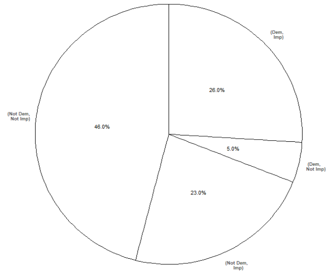
Figure 2.24: Spinner corresponding to Example 2.34.
There are two basic ways to use simulation to approximate a conditional probability \(\textrm{P}(A|B)\).
- Simulate the random phenomenon for a set number of repetitions (say 10000), discard those repetitions on which \(B\) does not occur, and compute the relative frequency of \(A\) among the remaining repetitions (on which \(B\) does occur).
- Disadvantage: the margin of error is based on only the number of repetitions used to compute the relative frequency. So if you perform 10000 repetitions but \(B\) occurs only on 2000, then the margin of error for estimate \(\textrm{P}(A|B)\) is roughly on the order of \(1/\sqrt{2000} = 0.022\) (rather than \(1/\sqrt{10000} = 0.01\). Especially if \(\textrm{P}(B)\) is small, the margin of error could be large resulting in an imprecise estimate of \(\textrm{P}(A|B)\).
- Advantage: not computationally intensive.
- Simulate the random phenomenon until obtaining a certain number of repetitions (say 10000) on which \(B\) occurs, discarding those repetitions on which \(B\) does not occur as you go, and compute the relative frequency of \(A\) among the remaining repetitions (on which \(B\) does occur).
- Advantage: the margin of error will be based on the set number of repetitions on which \(B\) occurs.
- Disadvantage: requires more time/computer power. Especially if \(\textrm{P}(B)\) is small, it will require a large number of repetitions of the simulation to achieve the desired number of repetitions on which \(B\) occurs.
In Symulate, filter can be used to extract repetitions that satisfy a condition. First we’ll simulate impeachment support status and party affiliation for 10000 hypothetical Americans.
Each ticket in the BoxModel has a (Support, Party) pair of labels, like the spinner in Figure 2.24.
P = BoxModel([('Support', 'Democrat'), ('Support', 'Not Democrat'), ('Not Support', 'Democrat'), ('Not Support', 'Not Democrat')],
             probs = [0.26, 0.23, 0.05, 0.46])

sim_all = P.sim(10000)

sim_all| Index | Result |
|---|---|
| 0 | ('Not Support', 'Not Democrat') |
| 1 | ('Support', 'Democrat') |
| 2 | ('Support', 'Not Democrat') |
| 3 | ('Not Support', 'Not Democrat') |
| 4 | ('Not Support', 'Not Democrat') |
| 5 | ('Not Support', 'Not Democrat') |
| 6 | ('Support', 'Democrat') |
| 7 | ('Not Support', 'Not Democrat') |
| 8 | ('Support', 'Democrat') |
| ... | ... |
| 9999 | ('Support', 'Not Democrat') |
sim_all.tabulate()| Outcome | Frequency |
|---|---|
| ('Not Support', 'Democrat') | 536 |
| ('Not Support', 'Not Democrat') | 4610 |
| ('Support', 'Democrat') | 2590 |
| ('Support', 'Not Democrat') | 2264 |
| Total | 10000 |
Now we’ll apply filter to retain only the Democrats.
The function is_Democrat takes as an input72 a (support status, party affiliation pair) and returns True if Democrat (and False otherwise).
Applying filter(is_Democrat) will only return results for which is_Democrat returns True.
def is_Democrat(Support_Party):
    return Support_Party[1] == 'Democrat'

sim_Dem = sim_all.filter(is_Democrat)

sim_Dem| Index | Result |
|---|---|
| 0 | ('Support', 'Democrat') |
| 1 | ('Support', 'Democrat') |
| 2 | ('Support', 'Democrat') |
| 3 | ('Support', 'Democrat') |
| 4 | ('Support', 'Democrat') |
| 5 | ('Support', 'Democrat') |
| 6 | ('Not Support', 'Democrat') |
| 7 | ('Support', 'Democrat') |
| 8 | ('Not Support', 'Democrat') |
| ... | ... |
| 3125 | ('Support', 'Democrat') |
sim_Dem.tabulate()| Outcome | Frequency |
|---|---|
| ('Not Support', 'Democrat') | 536 |
| ('Support', 'Democrat') | 2590 |
| Total | 3126 |
Conditional relative frequencies are computed based only on repetitions which satisfy the event being conditioned on.
sim_Dem.tabulate(normalize = True)| Outcome | Relative Frequency |
|---|---|
| ('Not Support', 'Democrat') | 0.17146513115802944 |
| ('Support', 'Democrat') | 0.8285348688419706 |
| Total | 1.0 |
In Symbulate, the given symbol | applies the second method to simulate a fixed number of repetitions that satisfy the event being conditioned on. Be careful when using | when conditioning on an event with small probability. In particular, be careful when conditioning on the value of a continuous random variable.
Below we use RV syntax to carry out the simulation and conditioning.
Technically, a random variable always returns a number, but RV in Symbulate does allow for non-numerical outputs.
In most situations, we will usually deal with true random variables, and the code syntax below will be more natural.
The following simulates (Support, Party) pairs until 10000 Democrats are obtained.
Support, Party = RV(P)

sim_Dem = ( (Support & Party) | (Party == 'Democrat') ).sim(10000)

sim_Dem| Index | Result |
|---|---|
| 0 | (Support, Democrat) |
| 1 | (Not Support, Democrat) |
| 2 | (Support, Democrat) |
| 3 | (Support, Democrat) |
| 4 | (Support, Democrat) |
| 5 | (Support, Democrat) |
| 6 | (Support, Democrat) |
| 7 | (Support, Democrat) |
| 8 | (Support, Democrat) |
| ... | ... |
| 9999 | (Not Support, Democrat) |
sim_Dem.tabulate()| Value | Frequency |
|---|---|
| (Not Support, Democrat) | 1649 |
| (Support, Democrat) | 8351 |
| Total | 10000 |
Since all 10000 simulated pairs satisfy the event being conditioned on (Democrat), they are all included in the computation of the conditional relative frequencies.
sim_Dem.tabulate(normalize = True)| Value | Relative Frequency |
|---|---|
| (Not Support, Democrat) | 0.1649 |
| (Support, Democrat) | 0.8351 |
| Total | 1.0 |
2.7.2 Joint, conditional, and marginal probabilities
Within the context of two events, we have joint, conditional, and marginal probabilities.
- Joint: unconditional probability involving both events, \(\textrm{P}(A \cap B)\).
- Conditional: conditional probability of one event given the other, \(\textrm{P}(A | B)\), \(\textrm{P}(B | A)\).
- Marginal: unconditional probability of a single event \(\textrm{P}(A)\), \(\textrm{P}(B)\).
The relationship \(\textrm{P}(A|B) = \textrm{P}(A\cap B)/\textrm{P}(B)\) can be stated generically as \[ \text{conditional} = \frac{\text{joint}}{\text{marginal}} \] We will see later that similar relationships are true for distributions of random variables.
In the previous impeachment problem, we were provided the joint and marginal probabilities and we computed conditional probabilities. But in many problems conditional probabilities are provided or can be determined directly.
Example 2.35 Recent polls73 suggest that
- 83% of Democrats support impeachment of President Trump
- 44% of Independents support impeachment of President Trump
- 14% of Republicans support impeachment of President Trump
The average of these three percentages is \((83+44+14)/3 = 47\). Is it necessarily true that 47% of all Americans support impeachment?
Based on recent polls74
- 31% of Americans are Democrats
- 40% of Americans are Independent
- 29% of Americans are Republicans
Define the event \(A\) to represent “supports impeachment” and \(D, I, R\) to correspond to affiliation in each of the parties. If the probability measure \(\textrm{P}\) corresponds to randomly selecting an American, write all the percentages above as probabilities using proper notation.
Find the probability that a randomly selected American is a Democrat who supports impeachment. Is this a joint, conditional, or marginal probability?
Construct an appropriate two-way table.
Find the probability that a randomly selected American supports impeachment. How does this differ from the average of the three percentages in part 1? Why?
Now suppose that the randomly selected American supports impeachment. How does this information change the probability that the selected American belongs to a particular political party? Answer by computing appropriate probabilities (and using proper notation).
How does each of the probabilities from the previous part compare to the respective prior probability? Does this make sense?
Solution. to Example 2.35
Show/hide solution
No, think of extreme cases as illustrations. If almost all of Americans were Democrats, then the overall probability of supporting impeachment would be close to 0.83, while if almost all of Americans were Republicans, then the overall probability of supporting impeachment would be close to 0.14. So the overall probability of supporting impeachment depends on the party affiliation breakdown.
If the probability measure \(\textrm{P}\) corresponds to randomly selecting an American then
- \(\textrm{P}(A|D) = 0.83\)
- \(\textrm{P}(A|I) = 0.44\)
- \(\textrm{P}(A|R) = 0.14\)
- \(\textrm{P}(D) = 0.31\)
- \(\textrm{P}(I) = 0.40\)
- \(\textrm{P}(R) = 0.29\)
The probability that a randomly selected American is a Democrat who supports impeachment is \(\textrm{P}(A \cap D) = \textrm{P}(A|D)\textrm{P}(D) = (0.83)(0.31) = 0.2573\), a joint probability. In 10000 hypothetical Americans, we would expect 3100 to be Democrats, and of those 3100 Democrats we would expect 2573 (or 83%) to support impeachment. So out of the 10000 Americans, 2573 are Democrats who support impeachment.
Continue in the manner of the previous part to complete a two-way table of counts for 10000 hypothetical Americans.
Impeach Not Impeach Total Democrat 2573 527 3100 Independent 1760 2240 4000 Republican 406 2494 2900 Total 4739 5261 10000 Out of the 10000 Americans, 4739 support impeachment, so the probability that a randomly selected American supports impeachment75 is \(\textrm{P}(A)=0.4739\). This is actually pretty close to the average of the 3 impeachment percentages, but that’s just a coincidence. The overall probability is actually a weighted average; in terms of the probabilities given in the setup, the table calculations show \[\begin{align*} \textrm{P}(A) & = \textrm{P}(A \cap D) + \textrm{P}(A \cap I) + \textrm{P}(A \cap R)\\ & = \textrm{P}(A|D)\textrm{P}(D) + \textrm{P}(A|I)\textrm{P}(I) + \textrm{P}(A|R)\textrm{P}(R)\\ & = (0.83)(0.31) + (0.44)(0.40) + (0.14)(0.29) \end{align*}\] This is an illustration of the “law of total probability”, which we will discuss in more detail soon.
We want \(\textrm{P}(D|A)\), etc.
- \(\textrm{P}(D|A) = \frac{2573}{4739} = \frac{(0.83)(0.31)}{(0.83)(0.31) + (0.44)(0.40) + (0.14)(0.29)} = 0.543\).
- \(\textrm{P}(I|A) = \frac{1760}{4739} = \frac{(0.44)(0.40)}{(0.83)(0.31) + (0.44)(0.40) + (0.14)(0.29)} = 0.371\).
- \(\textrm{P}(R|A) = \frac{406}{4739} = \frac{(0.14)(0.29)}{(0.83)(0.31) + (0.44)(0.40) + (0.14)(0.29)} = 0.086\). This is an illustration of “Bayes rule”, which we will discuss in more detail soon.
How does each of the probabilities from the previous part compare to the respective prior probability? Does this make sense?
- \(\textrm{P}(D|A) = 0.543\), which is greater than the prior probability of Democrat \(\textrm{P}(D) = 0.31\). Knowing the person supports impeachment increases the probability that the person is a Democrat.
- \(\textrm{P}(I|A) = 0.371\), which is slightly less than the prior probability of Independent \(\textrm{P}(I) = 0.40\). Knowing the person supports impeachment slightly decreases the probability that the person is an Independent.
- \(\textrm{P}(R|A) = 0.086\), which is less than the prior probability of Republican \(\textrm{P}(R) = 0.29\). Knowing the person supports impeachment decreases the probability that the person is a Republican.
A mosaic plot provides a nice visual of joint, marginal, and one-way conditional probabilities, and can be used to illustrate the law of total probability. The mosaic plot76 on the left in Figure 2.25 represents conditioning on political party. The vertical bars represent the conditional probabilities of supporting/not supporting impeachment for each political party. The widths of the vertical bars are scaled in proportion to the marginal distribution of party; the bar for Independent is a little wider than the others. The area of each sub-rectangle represents a joint probability. The single bar to the right of the plot displays the marginal probability of supporting/not supporting impeachment.
The plot on the right in Figure 2.25 represents conditioning on support of impeachment. Now the widths of the vertical bars represent the distribution of supporting/not supporting impeachment, the heights within the bars represent conditional probabilities for party affiliation given support status, and the single bar to the right represents the marginal distribution of party affiliation.
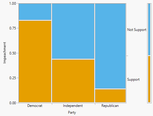
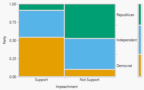
Figure 2.25: Mosaic plots for Example 2.35. The plot on the left represents conditioning on party affiliation, while the plot on the right represents conditioning on support for impeachment.
Example 2.36 Consider simulating a randomly selected American and determining whether or not the person supports impeachment and whether or not the person is a Democrat, as in the scenario in Example 2.35. Remember we are given \(\textrm{P}(A|D) = 0.83\), \(\textrm{P}(A|I) = 0.44\), \(\textrm{P}(A|R) = 0.14\), \(\textrm{P}(D) = 0.31\), \(\textrm{P}(I) = 0.40\), and \(\textrm{P}(R)=0.29\).
How could you perform one repetition of the simulation using spinners based solely on the probabilities provided in the problem, without first constructing a two-way table or finding \(\textrm{P}(A\cap B)\), etc? (Hint: you’ll need a few spinners, but you might not spin them all in a single repetition.)
Solution. to Example 2.36
Show/hide solution
There will be 4 spinners, but only 2 will be spun in any single repetition.
- “Party” spinner: Areas of 0.31, 0.40, and 0.29 correspond to, respectively, Democrat, Independent, Republican. Spin this to determine party affiliation.
- “Impeachment” spinners — only one of the following will be spun in a single repetition:
- Impeachment given Democrat: areas of 0.83 and 0.17 corresponding to, respectively, support, not support. If the result of the “party” spinner is Democrat, spin this spinner to determine support for impeachment.
- Impeachment given Independent: areas of 0.44 and 0.56 corresponding to, respectively, support, not support. If the result of the “party” spinner is Independent, spin this spinner to determine support for impeachment.
- Impeachment given Republican: areas of 0.14 and 0.86 corresponding to, respectively, support, not support. If the result of the “party” spinner is Republican, spin this spinner to determine support for impeachment.
We can code the above in Symbulate by defining a custom probability space. An outcome is a (party, impeachment) pair. Each of the 4 spinners corresponds to a BoxModel. We define a function that defines how to simulate one repetition, using the draw method. Then we use that function to define a custom ProbabilitySpace.
def party_impeachment_sim():
    party = BoxModel(['D', 'I', 'R'], probs = [0.31, 0.40, 0.29]).draw()
    if party == 'D':
        support = BoxModel(['Imp', 'NotImp'], probs = [0.83, 0.17]).draw()
    if party == 'I':
        support = BoxModel(['Imp', 'NotImp'], probs = [0.44, 0.56]).draw()
    if party == 'R':
        support = BoxModel(['Imp', 'NotImp'], probs = [0.14, 0.86]).draw()
    return party, support

P = ProbabilitySpace(party_impeachment_sim)
P.sim(10000).tabulate()| Outcome | Frequency |
|---|---|
| ('D', 'Imp') | 2653 |
| ('D', 'NotImp') | 497 |
| ('I', 'Imp') | 1750 |
| ('I', 'NotImp') | 2204 |
| ('R', 'Imp') | 388 |
| ('R', 'NotImp') | 2508 |
| Total | 10000 |
2.7.3 Multiplication rule
Rearranging the definition of conditional probability we get the Multiplication rule: the probability that two events both occur is
\[ \begin{aligned} \textrm{P}(A \cap B) & = \textrm{P}(A|B)\textrm{P}(B)\\ & = \textrm{P}(B|A)\textrm{P}(A) \end{aligned} \]
The multiplication rule says that you should think “multiply” when you see “and”. However, be careful about what you are multiplying: to find a joint probability you need an unconditional and an appropriate conditional probability. You can condition either on \(A\) or on \(B\), provided you have the appropriate marginal probability; often, conditioning one way is easier than the other. Be careful: the multiplication rule does not say that \(\textrm{P}(A\cap B)\) is the same as \(\textrm{P}(A)\textrm{P}(B)\).
For example:
- 31% of Americans are Democrats
- 83.9% of Democrats support impeachment
- So 26% of Americans are Democrats who support impeachment, \(0.26 = 0.31\times 0.839\).
\[ \frac{\text{Democrats who support impeachment}}{\text{Americans}} = \left(\frac{\text{Democrats}}{\text{Americans}}\right)\left(\frac{\text{Democrats who support impeachment}}{\text{Democrats}}\right) \]
Generically, the multiplication rule says \[ \text{joint} = \text{conditional}\times\text{marginal} \] We will see later that similar relationships are true for distributions of random variables.
2.7.4 Conditioning is “slicing and renormalizing”
The process of conditioning can be thought of as “slicing and renormalizing”.
- Extract the “slice” corresponding to the event being conditioned on (and discard the rest). For example, a slice might correspond to a particular row or column of a two-way table.
- “Renormalize” the values in the slice so that corresponding probabilities add up to 1.
We will see that the “slicing and renormalizing” interpretation also applies when dealing with conditional distributions of random variables, and corresponding plots. Slicing determines the shape; renormalizing determines the scale. Slicing determines relative probabilities; renormalizing just makes sure they add up to 1.
Example 2.37 Recall Example 2.32. Remember we are given \(\textrm{P}(A) = 0.49\), \(\textrm{P}(D) = 0.31\), and \(\textrm{P}(A\cap D) = 0.26\) where \(A\) is the event that the selected person supports impeachment and \(D\) is the event that the selected person is a Democrat.
- How many times more likely is it for an American to be a Democrat who supports impeachment than to be a Democrat who does not support impeachment?
- How many times more likely is it for a Democrat to support impeachment than to not support impeachment?
- What do you notice about the answers to the two previous parts?
Solution. to Example 2.37
Show/hide solution
- Note that the probability that an American is a Democrat who does not support impeachment is \(\textrm{P}(A^c \cap D) = \textrm{P}(D) - \textrm{P}(A\cap D) = 0.31 - 0.26 = 0.05\). The ratio in question is \(\frac{\textrm{P}(A \cap D)}{\textrm{P}(A^c \cap D)} = \frac{0.26}{0.05} = 5.2\). An American is 5.2 times more likely to be a Democrat who supports impeachment than to be a Democrat who does not support impeachment.
- Recall that \(\textrm{P}(A|D) = 0.839\) and \(\textrm{P}(A^c|D) = 0.161\). The ratio in question is \(\frac{\textrm{P}(A |D)}{\textrm{P}(A^c | D)} = \frac{0.839}{0.161} = 5.2\). A Democrat is 5.2 times more likely to support impeachment than to not support impeachment.
- The ratios are the same! Conditioning on Democrat just slices out the Americans who are Democrats. The ratios are determined by the overall probabilities for Americans, as in part 1. The conditional probabilities, given Democrat, in part 2 simply rescale the probabilities for Americans who are Democrats to add up to 1.
The following is a Venn diagram type example of slicing and renormalizing.
Example 2.38 Each of the three Venn diagrams below represents a sample space with 16 equally likely outcomes. Let \(A\) be the yellow / event, \(B\) the blue \ event, and their intersection \(A\cap B\) the green \(\times\) event. Suppose that areas represent probabilities, so that for example \(\textrm{P}(A) = 4/16\).
Find \(\textrm{P}(A|B)\) for each of the scenarios. Be sure to indicate what represents the “slice” in each scenario.
Solution. to Example 2.38
Show/hide solution
In each case, the slice represents the 4 blue outcomes.
- Left: \(\textrm{P}(A|B)=0\). After conditioning on \(B\), there are now 4 equally likely outcomes, of which none satisfy \(A\).
- Middle: \(\textrm{P}(A|B) = 2/4\). After conditioning on \(B\), there are now 4 equally likely outcomes, of which 2 satisfy \(A\).
- Right: \(\textrm{P}(A|B) = 1/4\). After conditioning on \(B\), there are now 4 equally likely outcomes, of which 1 satisfies \(A\).
2.7.5 Independence
In general, the conditional probability of event \(A\) given some other event \(B\) is usually different from the unconditional probability of \(A\). That is, in general \(\textrm{P}(A | B) \neq \textrm{P}(A)\). Knowledge of the occurrence of event \(B\) typically influences the probability of event \(A\), and vice versa. If so, we say that events \(A\) and \(B\) are dependent.
However, in some situations knowledge of the occurrence of one event does not influence the probability of another. For example, if a coin is flipped twice then knowing that the first flip landed on Heads does not change the probability that the second flips lands on Heads. In these situations we say the events are independent.
Example 2.39 Consider the following hypothetical data.
| Democrat (\(D\)) | Not Democrat (\(D^c\)) | Total | |
|---|---|---|---|
| Loves puppies (\(L\)) | 180 | 270 | 450 |
| Does not love puppies (\(L^c\)) | 20 | 30 | 50 |
| Total | 200 | 300 | 500 |
Suppose a person is randomly selected from this group. Consider the events \[\begin{align*} L & = \{\text{person loves puppies}\}\\ D & = \{\text{person is a Democrat}\} \end{align*}\]
- Compute and interpret \(\textrm{P}(L)\).
- Compute and interpret \(\textrm{P}(L|D)\).
- Compute and interpret \(\textrm{P}(L|D^c)\).
- What do you notice about \(\textrm{P}(L)\), \(\textrm{P}(L|D)\), and \(\textrm{P}(L|D^c)\)?
- Compute and interpret \(\textrm{P}(D)\).
- Compute and interpret \(\textrm{P}(D|L)\).
- Compute and interpret \(\textrm{P}(D|L^c)\).
- What do you notice about \(\textrm{P}(D)\), \(\textrm{P}(D|L)\), and \(\textrm{P}(D|L^c)\)?
- Compute and interpret \(\textrm{P}(D \cap L)\).
- What is the relationship between \(\textrm{P}(D \cap L\)) and \(\textrm{P}(D)\) and \(\textrm{P}(L)\)?
- When randomly selecting a person from this particular group, would you say that events \(D\) and \(L\) are independent? Why?
Solution. to Example 2.39
Show/hide solution
- The probability that the randomly selected person loves puppies is \(\textrm{P}(L)=450/500=0.9\).
- The conditional probability that the randomly selected person loves puppies given that the person is a Democrat is \(\textrm{P}(L|D)=180/200=0.9\).
- The conditional probability that the randomly selected person loves puppies given that the person is not a Democrat is \(\textrm{P}(L|D^c)=270/300=0.9\).
- \(\textrm{P}(L)=\textrm{P}(L|D)=\textrm{P}(L|D^c)=0.9\). Regardless of whether or not the person is a Democrat the probability that they love puppies is 0.9, the overall probability that a person loves puppies.
- The probability that the randomly selected person is a Democrat is \(\textrm{P}(D)=200/500=0.4\).
- The conditional probability that the randomly selected person is a Democrat given that the person loves puppies is \(\textrm{P}(D|L)=180/450=0.4\).
- The conditional probability that the randomly selected person is a Democrat given that the person does not love puppies is \(\textrm{P}(D|L^c)=20/50=0.4\).
- \(\textrm{P}(D)=\textrm{P}(D|L)=\textrm{P}(D|L^c)=0.4\). Regardless of whether or not the person loves puppies the probability that the person is a Democrat is 0.4, the overall probability that a person is a Democrat.
- The probability that the randomly selected person is a Democrat and loves puppies is \(\textrm{P}(D \cap L)=180/500=0.36\).
- \(\textrm{P}(D \cap L) = 0.36 = (0.4)(0.9)=\textrm{P}(D)\textrm{P}(L)\). The joint probability is a product of the marginal probabilities.
- Yes, the events \(D\) and \(L\) are independent. Knowing whether or not the person is a Democrat does not change the probability that the person loves puppies, and vice versa.
As in the example, events \(A\) and \(B\) are independent if the knowing whether or not one occurs does not change the probability of the other. For events \(A\) and \(B\) (with \(0<\textrm{P}(A)<1\) and \(0<\textrm{P}(B)<1\)) the following are equivalent. That is, if one is true then they all are true; if one is false, then they all are false.
\[\begin{align*} \text{$A$ and $B$} & \text{ are independent}\\ \textrm{P}(A \cap B) & = \textrm{P}(A)\textrm{P}(B)\\ \textrm{P}(A^c \cap B) & = \textrm{P}(A^c)\textrm{P}(B)\\ \textrm{P}(A \cap B^c) & = \textrm{P}(A)\textrm{P}(B^c)\\ \textrm{P}(A^c \cap B^c) & = \textrm{P}(A^c)\textrm{P}(B^c)\\ \textrm{P}(A|B) & = \textrm{P}(A)\\ \textrm{P}(A|B) & = \textrm{P}(A|B^c)\\ \textrm{P}(B|A) & = \textrm{P}(B)\\ \textrm{P}(B|A) & = \textrm{P}(B|A^c) \end{align*}\]
In general, the multiplication rule says \[\begin{align*} \textrm{P}(A \cap B) & = \textrm{P}(A|B)\textrm{P}(B)\\ \text{Joint} & = \text{Conditional}\times\text{Marginal} \end{align*}\]
For independent events, the multiplication rule simplifies
\[\begin{align*} \text{If $A$ and $B$ are independent then } && \textrm{P}(A \cap B) & = \textrm{P}(A)\textrm{P}(B)\\ \text{If independent then } && \text{Joint} & = \text{Product of Marginals} \end{align*}\]
The last statement above is why independence is represented by the product * syntax in Symbulate.
For example, in the meeting problem, if Regina’s arrival follows a Uniform(0, 60) model, Cady’s follows a Normal(30, 10) model, and they arrive independently of each other, we can simulate pairs of arrivals as follows; note the use of *.
P = Uniform(0, 60) * Normal(30, 10)
P.sim(5)| Index | Result |
|---|---|
| 0 | (28.314236760661455, 20.175499181411922) |
| 1 | (48.66477487946991, 34.420715423033066) |
| 2 | (17.33556223921267, 28.913579562469973) |
| 3 | (56.18468308231486, 21.78969375919441) |
| 4 | (45.10169962805362, 30.9727162645447) |
We can think of * as “spin each spinner independently, but what * really does is create a joint probability space as the product of two marginal probability spaces.
Example 2.40 Figure 2.26 displays four mosaic plots, each representing probabilities corresponding to two events \(A\) and \(B\). Which of the mosaic plots represent independent events?
Solution. to Example 2.40
Show/hide solution
The bottom two plots represent independent events. In these situations \(\textrm{P}(B|A) = \textrm{P}(B|A^c) = \textrm{P}(B)\).
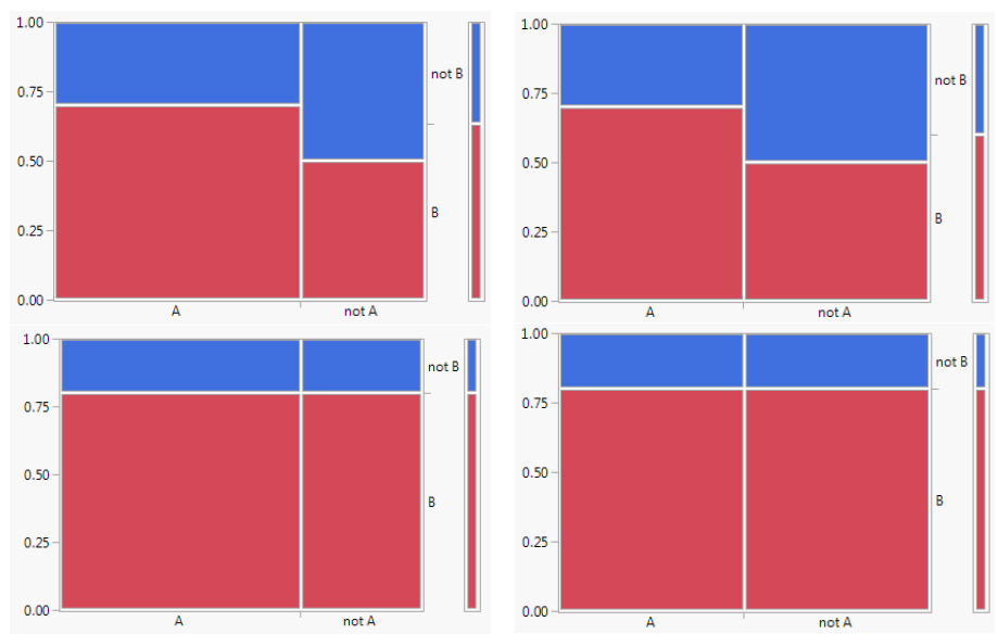
Figure 2.26: Four different mosaic plots for two events \(A\) and \(B\). In which of the plots are the events \(A\) and \(B\) independent?
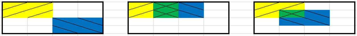
Example 2.41 Each of the three Venn diagrams below represents a sample space with 16 equally likely outcomes. Let \(A\) be the yellow / event, \(B\) the blue \ event, and their intersection \(A\cap B\) the green \(\times\) event. Suppose that areas represent probabilities, so that for example \(\textrm{P}(A) = 4/16\).
In which of the scenarios are events \(A\) and \(B\) independent?
Solution. to Example 2.41
Show/hide solution
In each case, \(\textrm{P}(A)=4/16\). Condition on event \(B\), by zooming in on the blue slice, and see if \(\textrm{P}(A|B)\) is the same as \(\textrm{P}(A)\).
- Left: \(\textrm{P}(A|B)=0\neq 4/16 = \textrm{P}(A)\). Therefore, events \(A\) and \(B\) are not independent.
- Middle: \(\textrm{P}(A|B) = 2/4\neq 4/16 = \textrm{P}(A)\). Therefore, events \(A\) and \(B\) are not independent.
- Right: \(\textrm{P}(A|B) = 1/4= 4/16 = \textrm{P}(A)\). Therefore, events \(A\) and \(B\) are independent. The ratio of yellow to total is the same as the ratio of the green part of blue to blue. If we zoom into the blue part of the picture (slice) and then resize it to the size of the original picture (renormalize), then the green part takes up 1/4 of the area just as the yellow part did in the original picture.
Do not confuse “disjoint” with “independent”. Disjoint means two events do not “overlap”. Independence means two events “overlap in just the right way”. You can pretty much forget “disjoint” exists; you will naturally apply the addition rule for disjoint events correctly without even thinking about it. Independence is much more important and useful, but also requires more care.
These number are estimates based on data from polls as of Oct 9, 2019. I wrote this exercise in Fall 2019. In Fall 2020, I decided not to change it, knowing that would make it outdated. But then Trump was impeached again in January 2021. And now we have the Jan 6 committee hearings.↩︎
Remember, this is a Simpsons reference, not a Trump reference.↩︎
The resulting value is estimated based on data from polls as of Oct 9, 2019 and party affiliation as of Sept 2019.↩︎
For the purposes of constructing a hypothetical table, it doesn’t matter what value you use for the total, as long as you don’t round any of the counts in the interior cells. If interior cells are decimals, either leave them as decimals, or add a few zeros to the total count and redo.↩︎
Provided \(\textrm{P}(B)>0\). We will assume throughout that all events being conditioned on have non-zero probability. We will discuss some issues related to conditioning on the value of a continuous random variable later.↩︎
Support_Partyis a pair soSupport_Party[0]is the first component (Support) andSupport_Party[1]is the second component (Party).↩︎This number differs from the one in the previous impeachment problem because of rounding errors in the probabilities reported in the setups.↩︎
Unfortunately, mosaic plots are not available in Symbulate yet.↩︎