6.4 Poisson distributions

Example 6.15 Let $X$ be the number of home runs hit (in total by both teams) in a randomly selected Major League Baseball game.

1. In what ways is this like the Binomial situation? (What is a trial? What is “success”?)
2. In what ways is this NOT like the Binomial situation?

Solution. to Example 6.15

Show/hide solution

1. Each pitch is a trial, and on each trial either a home run is hit (“success”) or not. The random variable $X$ counts the number of home runs (successes) over all the trials
2. Even though $X$ is counting successes, this is not the Binomial situation.
   • The number of trials is not fixed. The total number of pitches varies from game to game. (The average is around 300 pitches per game).
   • The probability of success is not the same on each trial. Different batters have different probabilities of hitting home runs. Also, different pitch counts or game situations lead to different probabilities of home runs.
   • The trials might not be independent, though this is a little more questionable. Make sure you distinguish independence from the previous assumption of unequal probabilities of success; you need to consider conditional probabilities to assess independence. Maybe if a pitcher gives up a home run on one pitch, then the pitcher is “rattled” so the probability that he also gives up a home run on the next pitch increases, or the pitcher gets pulled for a new pitcher which changes the probability of a home run on the next pitch.

Example 6.16 Let $X$ be the number of automobiles that get in accidents on Highway 101 in San Luis Obispo on a randomly selected day.

1. In what ways is this like the Binomial situation? (What is a trial? What is “success”?)

2. In what ways is this NOT like the Binomial situation?

3. Which of the following do you think it would be easier to estimate by collecting and analyzing relevant data?

   • The total number of cars on the highway each day, and the probability that each driver on the highway has an accident.
   • The average number of accidents per day that happen on the highway.

Solution. to Example 6.16

Show/hide solution

1. Each automobile on the road in the day is a trial, and each automobile either gets in an accident (“success”) or not. The random variable $X$ counts the number of automobiles that get into accidents (successes). (Remember “success” is just a generic label for the event you’re interested in; “success” is not necessarily good.)
2. Even though $X$ is counting successes, this is not the Binomial situation.
   • The number of trials is not fixed. The total number of automobiles on the road varies from day to day.
   • The probability of success is not the same on each trial. Different drivers have different probabilities of getting into accidents; some drivers are safer than others. Also, different conditions increase the probability of an accident, like driving at night.
   • The trials are plausibly not independent. Make sure you distinguish independence from the previous assumption of unequal probabilities of success; you need to consider conditional probabilities to assess independence. If an automobile gets into an accident, then the probability of getting into an accident increases for the automobiles that are driving near it.
3. It would be very difficult to estimate the probability that each individual driver gets into an accident. (Though you probably could measure the total number of cars.) It would be much easier to find data on total number of accidents that happen each day over some period of time, e.g., from police reports, and use it to estimate the average number of accidents per day.

The Binomial model has several restrictive assumptions that might not be satisfied in practice

• The number of trials must be fixed (not random) and known.
• The probability of success must be the same for each trial (fixed, not random) and known.
• The trials must be independent.

Even when the trials are independent with the same probability of success, fitting a Binomial model to data requires estimation of both $n$ and $p$ individually, rather than just the mean $\mu=np$. When the only data available are success counts (e.g., number of accidents per day for a sample of days) $\mu$ can be estimated but $n$ and $p$ individually cannot.

Poisson models are more flexible models for counts. Poisson models are parameterized by a single parameter (the mean) and do not require all the assumptions of a Binomial model. Poisson distributions are often used to model the distribution of random variables that count the number of “relatively rare” events that occur over a certain interval of time in a certain region (e.g., number of accidents on a highway in a day, number of car insurance policies that have claims in a week, number of bank loans that go into default, number of mutations in a DNA sequence, number of earthquakes that occurs in SoCal in an hour, etc.)

Definition 6.5 A discrete random variable $X$ has a Poisson distribution with parameter¹³² $\mu>0$ if its probability mass function $p_X$ satisfies $$\begin{align*} p_X(x) & \propto \frac{\mu^x}{x!}, \;\qquad x=0,1,2,\ldots\\ & = \frac{e^{-\mu}\mu^x}{x!}, \quad x=0,1,2,\ldots \end{align*}$$ If $X$ has a Poisson($\mu$) distribution then $$\begin{align*} \textrm{E}(X) & = \mu\\ \textrm{Var}(X) & = \mu \end{align*}$$

The shape of a Poisson pmf as a function of $x$ is given by $\mu^x/x!$. The constant $e^{-\mu}$ simply renormalizes the heights of the pmf so that the probabilities sum to 1. Recall the Taylor series expansion: $e^{\mu} = \sum_{x=0}^\infty \frac{\mu^x}{x!}$.

For a Poisson distribution, both the mean and variance are equal to $\mu$, but remember that the mean is measured in the count units (e.g., home runs) but the variance is measured in squared units (e.g., $(\text{home runs})^2$).

Poisson(0.3).plot()
Poisson(1).plot()
Poisson(2).plot()
plt.legend(['Poisson(0.3)', 'Poisson(1)', 'Poisson(2)']);
plt.show()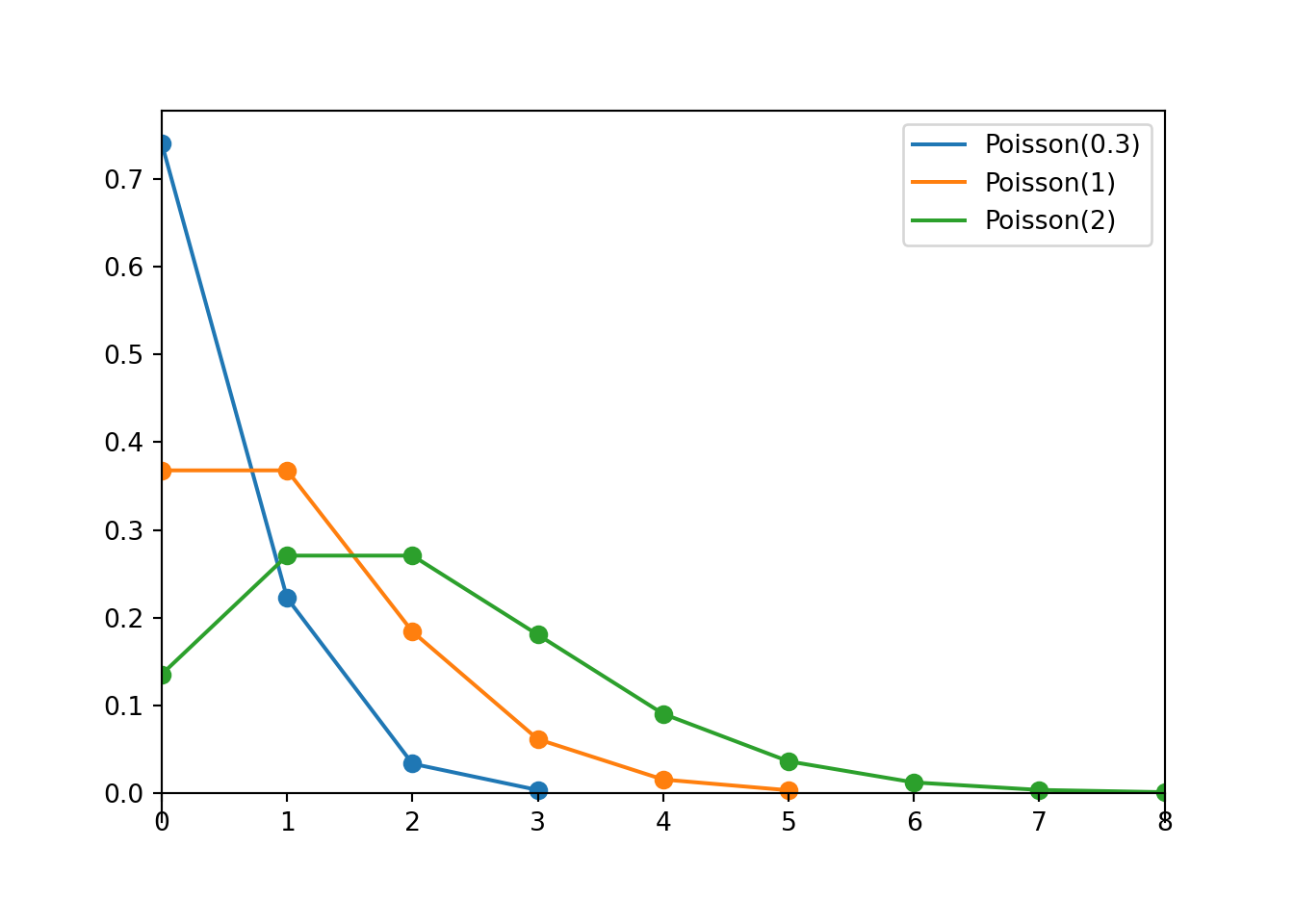

Example 6.17 Suppose that the number of typographical errors on a randomly selected page of a textbook has a Poisson distribution with parameter $\mu = 0.3$.

1. Find the probability that a randomly selected page has no typographical errors.
2. Find the probability that a randomly selected page has exactly one typographical error.
3. Find the probability that a randomly selected page has exactly two typographical errors.
4. Find the probability that a randomly selected page has at least three typographical errors.
5. Provide a long run interpretation of the parameter $\mu=0.3$.
6. Suppose that each page in the book contains exactly 2000 characters and that the probability that any single character is a typo is 0.00015, independently of all other characters. Let $X$ be the number of characters on a randomly selected page that are typos. Identify the distribution of $X$ and its expected value and variance, and compare to a Poisson(0.3) distribution.

Solution. to Example 6.17

Show/hide solution

Let $X$ be the number of typos. Then the pmf of $X$ is $$p_X(x) = \frac{e^{-0.3}0.3^x}{x!}, \qquad x = 0, 1, 2, \ldots$$

1. Find the probability that a randomly selected page has no typographical errors.
   $$\textrm{P}(X = 0) = p_X(0) = \frac{e^{-0.3}0.3^0}{0!} = e^{-0.3} = 0.741$$

   About 74.1% of pages have no typos.

2. Find the probability that a randomly selected page has exactly one typographical error. $$\textrm{P}(X = 1) = p_X(1) = \frac{e^{-0.3}0.3^1}{1!} = 0.3e^{-0.3} = 0.222$$

   About 22.2% of pages have exactly 1 typo.

3. Find the probability that a randomly selected page has exactly two typographical errors. $$\textrm{P}(X = 2) = p_X(2) = \frac{e^{-0.3}0.3^2}{2!} = 0.033$$

   About 3.3% of pages have exactly 2 typos.

4. Find the probability that a randomly selected page has at least three typographical errors. $$\textrm{P}(X \ge 3) = 1 - \textrm{P}(X \le 2) = 1 - (0.741 + 0.222 + 0.033) = 0.0036$$

   About 0.36% of pages have at least 3 typos.

5. Provide a long run interpretation of the parameter $\mu=0.3$.

   There are 0.3 typos per page on average.

6. Suppose that each page in the book contains exactly 2000 characters and that the probability that any single character is a typo is 0.00015, independently of all other characters. Let $X$ be the number of characters on a randomly selected page that are typos. Identify the distribution of $X$ and its expected value and variance, and compare to a Poisson(0.3) distribution.

   In this case $X$ has a Binomial(2000, 0.00015) distribution with mean $2000(0.00015) = 0.3$ and variance $2000(0.00015)(1-0.00015) = 0.299955 \approx 0.3 = 2000(0.00015)$. See below for a simulation; the Binomial(2000, 0.00015) is very similar to the Poisson(0.3) distribution.

X = RV(Poisson(0.3))

x = X.sim(10000)

x.plot('impulse')

Poisson(0.3).plot()

plt.show()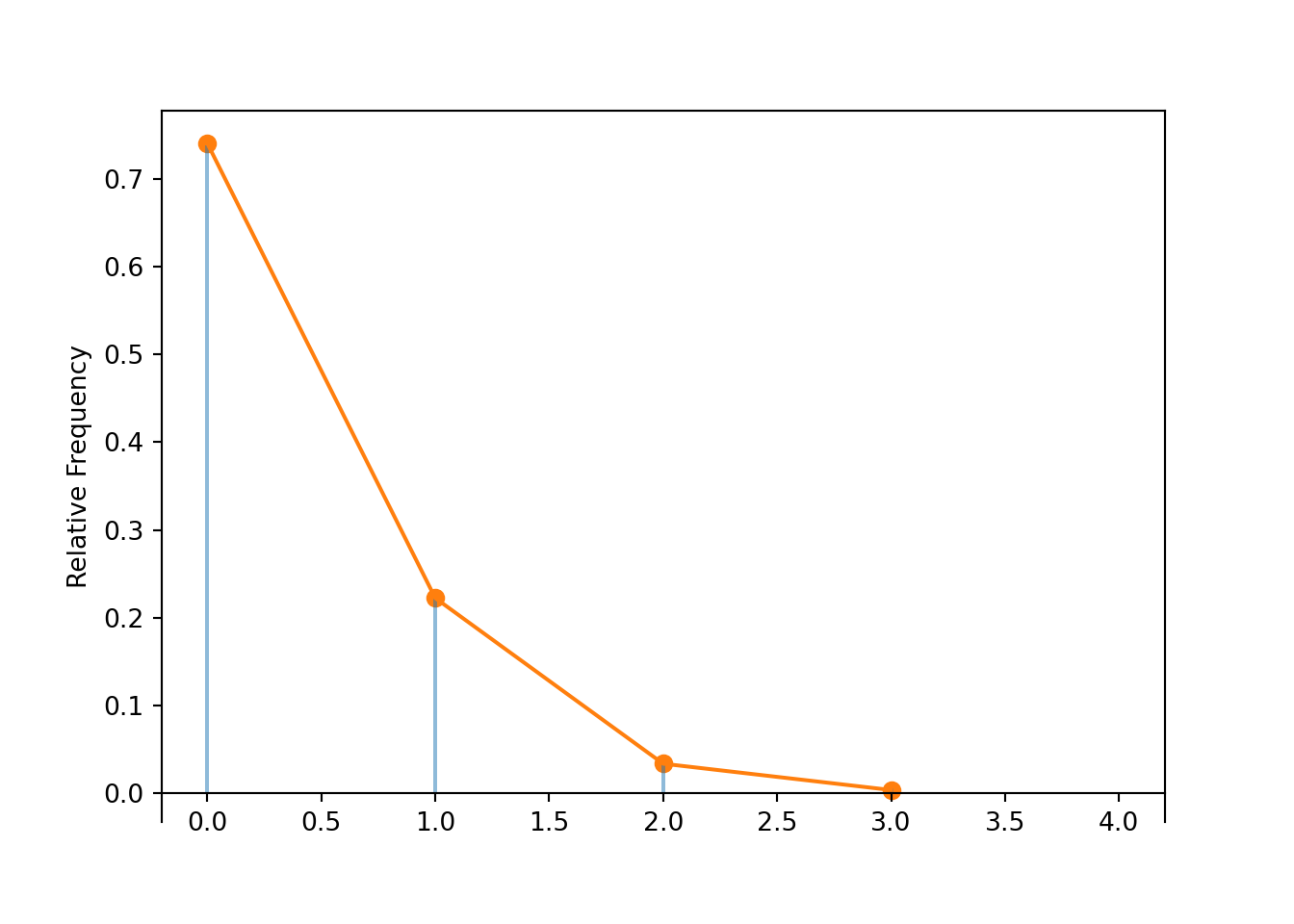

x.tabulate(normalize = True)

Value	Relative Frequency
0	0.7388
1	0.2213
2	0.0347
3	0.0049
4	0.0003
Total	0.9999999999999999

x.count_eq(0) / 10000, Poisson(0.3).pmf(0)

## (0.7388, 0.7408182206817179)

x.count_leq(2) / 10000, Poisson(0.3).cdf(2)

## (0.9948, 0.9964005068169105)

x.mean(), Poisson(0.3).mean()

## (0.3066, 0.3)

x.var(), Poisson(0.3).var()

## (0.31499644, 0.3)

RV(Binomial(2000, 0.00015)).sim(10000).plot('impulse')

Poisson(0.3).plot()

plt.show()

Example 6.18 Suppose $X_1$ and $X_2$ are independent, each having a Poisson(1) distribution, and let $X=X_1+X_2$. Also suppose $Y$ has a Poisson(2) distribution. For example suppose that $(X_1, X_2)$ represents the number of home runs hit by the (home, away) team in a baseball game, so $X$ is the total number of home runs hit by either team in the game, and $Y$ is the number of accidents that occur in a day on a particular stretch of highway

1. How could you use a spinner to simulate a value of $X$? Of $Y$? Are $X$ and $Y$ the same variable?
2. Compute $\textrm{P}(X=0)$. (Hint: what $(X_1, X_2)$ pairs yield $X=0$). Compare to $\textrm{P}(Y=0)$.
3. Compute $\textrm{P}(X=1)$. (Hint: what $(X_1, X_2)$ pairs yield $X=1$). Compare to $\textrm{P}(Y=1)$.
4. Compute $\textrm{P}(X=2)$. (Hint: what $(X_1, X_2)$ pairs yield $X=2$). Compare to $\textrm{P}(Y=2)$.
5. Are $X$ and $Y$ the same variable? Do $X$ and $Y$ have the same distribution?

Solution. to Example 6.18

Show/hide solution

1. How could you use a spinner to simulate a value of $X$? Of $Y$? Are $X$ and $Y$ the same variable? To generate a value of $X$: Construct a spinner corresponding to Poisson(1) distribution (see Figure 6.5), spin it twice and add the values together. To generate a value of $Y$: construct a spinner corresponding to a Poisson(2) distribution and spin it once (see Figure 6.6). $X$ and $Y$ are not the same random variable; they are measuring different things. The sum of two spins of the Poisson(1) spinner does not have to be equal to the result of the spin of the Poisson(2) spinner.

2. Compute $\textrm{P}(X=0)$. (Hint: what $(X_1, X_2)$ pairs yield $X=0$). Compare to $\textrm{P}(Y=0)$. The only way $X$ can be 0 is if both $X_1$ and $X_2$ are 0. $$\begin{align*} \textrm{P}(X = 0) & = \textrm{P}(X_1 = 0, X_2 = 0) & &\\ & = \textrm{P}(X_1 = 0)\textrm{P}(X_2 = 0) & & \text{independence}\\ & = \left(\frac{e^{-1}1^0}{0!}\right)\left(\frac{e^{-1}1^0}{0!}\right) & & \text{Poisson(1) pmf of $X_1, X_2$}\\ & = (0.368)(0.368) = 0.135 & & \\ & = \frac{e^{-2}2^0}{0!} & & \text{algebra} \\ & = \textrm{P}(Y = 0) & & \text{Poisson(2) pmf of $Y$} \end{align*}$$

3. Compute $\textrm{P}(X=1)$. (Hint: what $(X_1, X_2)$ pairs yield $X=1$). Compare to $\textrm{P}(Y=1)$. The only way $X$ can be 1 is if $X_1=1, X_2 = 0$ or $X_1 = 0, X_2=1$. $$\begin{align*} \textrm{P}(X = 1) & = \textrm{P}(X_1 = 1, X_2 = 0) + \textrm{P}(X_1 = 0, X_2 = 1)& &\\ & = \textrm{P}(X_1 = 1)\textrm{P}(X_2 = 0) + \textrm{P}(X_1 = 0)\textrm{P}(X_2 = 1) & & \text{independence}\\ & = 2\left(\frac{e^{-1}1^1}{1!}\right)\left(\frac{e^{-1}1^0}{0!}\right) & & \text{Poisson(1) pmf of $X_1, X_2$}\\ & = 2(0.368)(0.368) = 0.271 & & \\ & = \frac{e^{-2}2^1}{1!} & & \text{algebra} \\ & = \textrm{P}(Y = 1) & & \text{Poisson(2) pmf of $Y$} \end{align*}$$

4. Compute $\textrm{P}(X=2)$. (Hint: what $(X_1, X_2)$ pairs yield $X=2$). Compare to $\textrm{P}(Y=2)$. The only way $X$ can be 2 is if $X_1=2, X_2 = 0$ or $X_1 = 1, X_2=1$ or $X_1=0, X_2 = 2$. $$\begin{align*} \textrm{P}(X = 2) & = \textrm{P}(X_1 = 2, X_2 = 0) + \textrm{P}(X_1 = 1, X_2 = 1) + \textrm{P}(X_1 = 0, X_2 = 2)& &\\ & = \textrm{P}(X_1 = 2)\textrm{P}(X_2 = 0) + \textrm{P}(X_1 = 1)\textrm{P}(X_2 = 1) + \textrm{P}(X_1 = 0)\textrm{P}(X_2 = 2)& & \text{independence}\\ & = 2\left(\frac{e^{-1}1^2}{2!}\right)\left(\frac{e^{-1}1^0}{0!}\right) + \left(\frac{e^{-1}1^1}{1!}\right)\left(\frac{e^{-1}1^1}{1!}\right) & & \text{Poisson(1) pmf of $X_1, X_2$}\\ & = 2(0.184)(0.368) + (0.368)(0.368)= 0.271 & & \\ & = \frac{e^{-2}2^2}{2!} & & \text{algebra} \\ & = \textrm{P}(Y = 2) & & \text{Poisson(2) pmf of $Y$} \end{align*}$$

5. Are $X$ and $Y$ the same variable? Do $X$ and $Y$ have the same distribution? We already said that $X$ and $Y$ are not the same random variable. But the above calculations suggest that $X$ and $Y$ do have the same distributions. See the simulation results below.

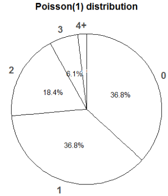
Figure 6.5: Spinner corresponding to a Poisson(1) distribution.

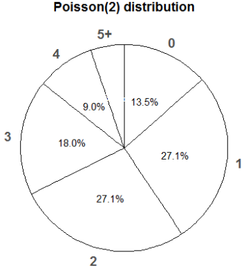
Figure 6.6: Spinner corresponding to a Poisson(2) distribution.

X1, X2 = RV(Poisson(1) ** 2)
X = X1 + X2

X.sim(10000).plot()

Poisson(2).plot()
plt.show()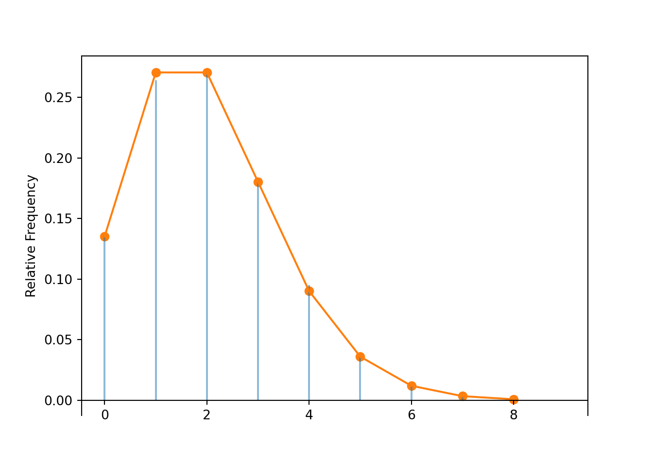

Poisson aggregation. If $X$ and $Y$ are independent, $X$ has a Poisson($\mu_X$) distribution, and $Y$ has a Poisson($\mu_Y$) distribution, then $X+Y$ has a Poisson($\mu_X+\mu_Y$) distribution.

If $X$ has mean $\mu_X$ and $Y$ has mean $\mu_Y$ then linearity of expected value implies that $X+Y$ has mean $\mu_X + \mu_Y$. If $X$ has variance $\mu_X$ and $Y$ has variance $\mu_Y$ then independence of $X$ and $Y$ implies that $X+Y$ has variance $\mu_X + \mu_Y$. What Poisson aggregation says is that if component counts are independent and each has a Poisson distribution, then the total count also has a Poisson distribution.

Here’s one proof involving law of total probability¹³³: We want to show that $p_{X+Y}(z) = \frac{e^{-(\mu_X+\mu_Y)}(\mu_X+\mu_Y)^z}{z!}$ for $z=0,1,2,\ldots$ $$\begin{align*} \textrm{P}(X+Y=z) & \stackrel{\text{(LTP)}}{=} \sum_{x=0}^\infty \textrm{P}(X=x,X+Y=z) = \sum_{x=0}^z \textrm{P}(X=x,Y=z-x) \\ & \stackrel{\text{(indep.)}}{=} \sum_{x=0}^z \textrm{P}(X=x)\textrm{P}(Y=z-x)\\ & = \sum_{x=0}^z \left(\frac{e^{-\mu_X}\mu_X^x}{x!}\right)\left(\frac{e^{-\mu_Y}\mu_Y^{z-x}}{(z-x)!}\right)\\ & \stackrel{\text{(algebra)}}{=} \frac{e^{-(\mu_X+\mu_Y)}(\mu_X+\mu_Y)^z}{z!}\sum_{x=0}^z\frac{z!}{x!(z-x)!}\left(\frac{\mu_X}{\mu_X+\mu_Y}\right)^x\left(1-\frac{\mu_X}{\mu_X+\mu_Y}\right)^{z-x}\\ & \stackrel{\text{(binom.)}}{=} \frac{e^{-(\mu_X+\mu_Y)}(\mu_X+\mu_Y)^z}{z!} \end{align*}$$

Example 6.19 Suppose $X$ and $Y$ are independent with $X\sim\text{Poisson}(1)$ and $Y\sim\text{Poisson}(2)$. For example, suppose $(X, Y)$ represents the number of goals scored by the (away, home) team in a soccer game.

1. How could you use spinners to simulate the conditional distribution of $X$ given $\{X+Y=2\}$?
2. Are the random variables $X$ and $X + Y$ independent?
3. Compute $\textrm{P}(X=0|X+Y=2)$.
4. Compute $\textrm{P}(X=1|X+Y=2)$.
5. Compute $\textrm{P}(X=x|X+Y=2)$ for all other possible values of $x$.
6. Identify the conditional distribution of $X$ given $\{X+Y=2\}$.
7. Compute $\textrm{E}(X | X+Y=2)$.

Solution. to Example 6.19

Show/hide solution

1. How could you use spinners to simulate the conditional distribution of $X$ given $\{X+Y=2\}$?

   • Spin the Poisson(1) spinner once to generate $X$.
   • Spin the Poisson(2) spinner once to generate $Y$.
   • Compute $X + Y$. If $X + Y = 2$ keep and record $X$; otherwise discard the repetition.
   • Repeat many times to simulate many values of $X$ given $X + Y = 2$. Summarize the simulated values of $X$ and their simulated relative frequencies to approximate the conditional distribution of $X$ given $\{X + Y = 2\}$.

2. Are the random variables $X$ and $X + Y$ independent? No. For example, $\textrm{P}(X =0)<1$ but $\textrm{P}(X = 0 | X + Y = 0) = 1$.

3. Compute $\textrm{P}(X=0|X+Y=2)$. The key is to take advantage of the fact that while $X$ and $X+Y$ are not independent, $X$ and $Y$ are. Write events involving $X$ and $X+Y$ in terms of equivalent events involving $X$ and $Y$. For example, the event $\{X = 0, X+ Y = 2\}$ is the same as the event $\{X = 0, Y = 2\}$. Also, remember that by Poisson aggregation $(X+Y)$ has a Poisson(3) distribution.

   $$\begin{align*} \textrm{P}(X = 0 | X + Y = 2) & = \frac{\textrm{P}(X = 0, X + Y = 2)}{\textrm{P}(X + Y = 2)} & & \text{definition of CP}\\ & = \frac{\textrm{P}(X = 0, Y = 2)}{\textrm{P}(X + Y = 2)} & & \text{same events}\\ & = \frac{\textrm{P}(X = 0)\textrm{P}(Y = 2)}{\textrm{P}(X + Y = 2)} & & \text{independence of $X$ and $Y$}\\ & = \frac{\left(\frac{e^{-1}1^0}{0!}\right)\left(\frac{e^{-2}2^2}{2!}\right)}{\left(\frac{e^{-3}3^2}{2!}\right)} & & \text{Poisson pmfs of $X$, $Y$, and $X+Y$}\\ & = \binom{2}{0}\left(\frac{1}{1+2}\right)^0\left(1-\frac{1}{1+2}\right)^2 & & \text{algebra} \\ & = 0.444 \end{align*}$$

4. Compute $\textrm{P}(X=1|X+Y=2)$.

   $$\begin{align*} \textrm{P}(X = 1 | X + Y = 2) & = \frac{\textrm{P}(X = 1, X + Y = 2)}{\textrm{P}(X + Y = 2)} & & \text{definition of CP}\\ & = \frac{\textrm{P}(X = 1, Y = 1)}{\textrm{P}(X + Y = 2)} & & \text{same events}\\ & = \frac{\textrm{P}(X = 1)\textrm{P}(Y = 1)}{\textrm{P}(X + Y = 2)} & & \text{independence of $X$ and $Y$}\\ & = \frac{\left(\frac{e^{-1}1^1}{1!}\right)\left(\frac{e^{-2}2^1}{1!}\right)}{\left(\frac{e^{-3}3^2}{2!}\right)} & & \text{Poisson pmfs of $X$, $Y$, and $X+Y$}\\ & = \binom{2}{1}\left(\frac{1}{1+2}\right)^1\left(1-\frac{1}{1+2}\right)^1 & & \text{algebra} \\ & = 0.444 \end{align*}$$

5. Compute $\textrm{P}(X=x|X+Y=2)$ for all other possible values of $x$.

   Given $X+Y=2$, the only possible values of $X$ are 0, 1, 2. So we just need to find $\textrm{P}(X = 2|X + Y = 2)$. We could just use the fact that the probabilities must sum to 1, but here is the long calculation to help you see the pattern.

   $$\begin{align*} \textrm{P}(X = 2 | X + Y = 2) & = \frac{\textrm{P}(X = 2, X + Y = 2)}{\textrm{P}(X + Y = 2)} & & \text{definition of CP}\\ & = \frac{\textrm{P}(X = 2, Y = 0)}{\textrm{P}(X + Y = 2)} & & \text{same events}\\ & = \frac{\textrm{P}(X = 2)\textrm{P}(Y = 0)}{\textrm{P}(X + Y = 2)} & & \text{independence of $X$ and $Y$}\\ & = \frac{\left(\frac{e^{-1}1^2}{2!}\right)\left(\frac{e^{-2}2^0}{0!}\right)}{\left(\frac{e^{-3}3^2}{2!}\right)} & & \text{Poisson pmfs of $X$, $Y$, and $X+Y$}\\ & = \binom{2}{2}\left(\frac{1}{1+2}\right)^2\left(1-\frac{1}{1+2}\right)^0 & & \text{algebra} \\ & = 0.111 \end{align*}$$

6. Identify the conditional distribution of $X$ given $\{X+Y=2\}$. The calculations above suggest that the conditional distribution of $X$ given $\{X + Y = 2\}$ is the Binomial distribution with $n=2$ and $p=\frac{1}{1+2} = \frac{\mu_X}{\mu_X+\mu_Y}$

7. Compute $\textrm{E}(X | X+Y=2)$. We could use the distribution and the definition: $\textrm{E}(X | X+Y=2) = 0(0.444) + 1(0.444) + 2(0.111) = 2/3$. Also, the conditional distribution of $X$ given $\{X + Y = 2\}$ is Binomial(2, 1/3), which has mean 2(1/3), so $\textrm{E}(X | X+Y=2)=2/3$.

X, Y = RV(Poisson(1) * Poisson(2))

x_given_Zeq2 = (X | (X + Y == 2)).sim(10000)

x_given_Zeq2.tabulate()

Value	Frequency
0	4478
1	4450
2	1072
Total	10000

x_given_Zeq2.mean()

## 0.6594

x_given_Zeq2.plot()

Binomial(2, 1 / 3).plot()
plt.show()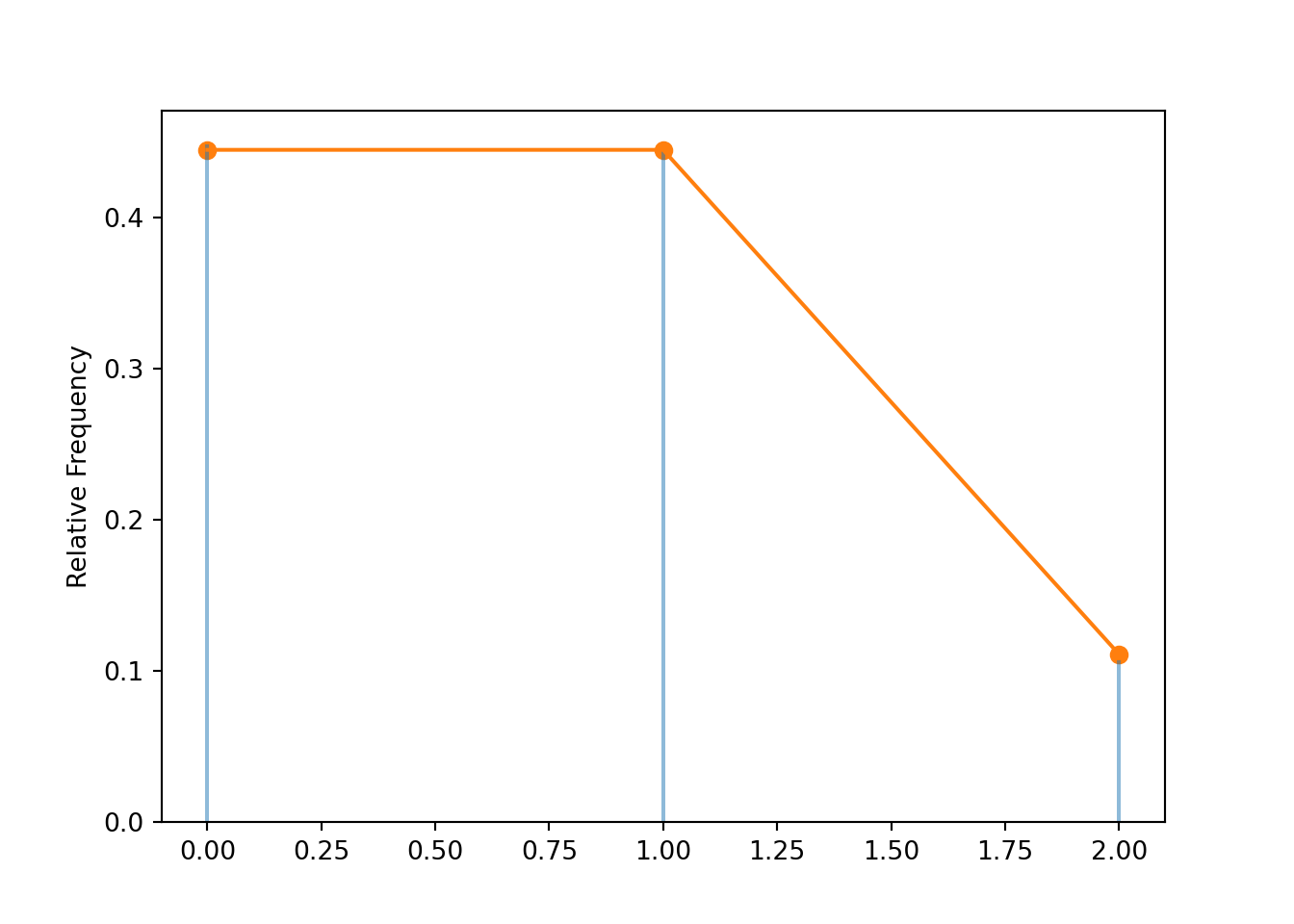

Poisson disaggregation (a.k.a., splitting, a.k.a., thinning). If $X$ and $Y$ are independent, $X$ has a Poisson($\mu_X$) distribution, and $Y$ has a Poisson($\mu_Y$) distribution, then the conditional distribution of $X$ given $\{X+Y=n\}$ is Binomial $\left(n, \frac{\mu_X}{\mu_X+\mu_Y}\right)$.

The total count of occurrences $X+Y=n$ can be disaggregated into counts for occurrences of “type $X$” or occurrences of “type $Y$”. Given $n$ occurrences in total, each of the $n$ occurrences is classified as type $X$ with probability proportional to the mean number of occurrences of type $X$, $\frac{\mu_X}{\mu_X+\mu_Y}$, and occurrences are classified independently of each other.

6.4.1 Poisson approximation

Where do Poisson distributions come from? We saw in Example 6.17 that the Binomial(2000, 0.00015) distribution is approximately the Poisson(0.3) distribution. This is an example of the “Poisson approximation to the Binomial”. If $X$ counts the number of successes in a Binomial situation where the number of trials $n$ is large and the probability of success on any trial $p$ is small, then $X$ has an approximate Poisson distribution with parameter $np$.

Let’s see why. We’ll reparametrize the Binomial($2000, 0.00015$) pmf in terms of the mean $0.3$, and apply some algebra and some approximations. Remember, the pmf is a distribution on values of the count $x$, for $x=0, 1, 2, \ldots$, but the probabilities are negligible if $x$ is not small.

$$\begin{align*} & \quad \binom{2000}{x}0.00015^x(1-0.00015)^{2000-x}\\ = & \quad \frac{2000!}{x!(2000-x)!}\frac{0.3^x}{2000^x}\left(1-\frac{0.3}{2000}\right)^{2000}(1-0.00015)^{-x} & & \text{algebra, $0.00015=0.3/2000$}\\ = & \quad \frac{2000(2000-1)(2000-2)\cdots(2000-x+1)}{(2000)(2000)(2000)\cdots(2000)}\frac{0.3^x}{x!}\left(1-\frac{0.3}{2000}\right)^{2000}(1-0.00015)^{-x} & & \text{algebra, rearranging}\\ = & \quad \left(1-\frac{1}{2000}\right)\left(1-\frac{2}{2000}\right)\cdots\left(1-\frac{x-1}{2000}\right)\frac{0.3^x}{x!}(0.7408)(1-0.00015)^{-x} & & \text{algebra, rearranging}\\ \approx & \quad (1)\frac{0.3^x}{x!}(0.7408)(1) & & \text{approximating, for $x$ small}\\ \approx & \quad e^{-0.3} \frac{0.3^x}{x!} \end{align*}$$

The above calculation shows that the Binomial(2000, 0.3) pmf is approximately equal to the Poisson(0.3) pmf.

Now we’ll consider a general Binomial situation. Let $X$ count the number of successes in $n$ Bernoulli($p$) trials, so $X$ has a Binomial($n$,$p$) distribution. Suppose that $n$ is “large”, $p$ is “small” (so success is “rare”) and $np$ is “moderate”. Then $X$ has an approximate Poisson distribution with mean $np$. The following states this idea more formally. The limits in the following make precise the notions of “large” ($n\to \infty$), “small” ($p_n\to 0$), and “moderate” ($np_n\to \mu \in (0,\infty)$).

Poisson approximation to Binomial. Consider $n$ Bernoulli trials with probability of success on each trial¹³⁴ equal to $p_n$. Suppose that $n\to\infty$ while $p_n\to0$ and $np_n\to\mu$, where $0<\mu<\infty$. Then for $x=0,1,2,\ldots$ $$\lim_{n\to\infty} \binom{n}{x} p_n^x \left(1-p_n\right)^{n-x} = \frac{e^{-\mu}\mu^x}{x!}$$

The proof relies on the same ideas we used in the Binomial(2000, 0.00015) approximation above. Fix $x=0,1,2,\ldots$ (Since we are letting $n\to\infty$ we can assume that $n>x$.) Some algebra and rearranging yields $$\begin{align*} \binom{n}{x} p_n^x \left(1-p_n\right)^{n-x} &= \left(\frac{n!}{x!(n-x)!}\right)\left(\frac{np_n}{n}\right)^x\left(1-p_n\right)^n\left(1-p_n\right)^{-x}\\ & = \left(\frac{n(n-1)(n-2)\cdots(n-x+1)}{n^x}\right)\left(\frac{\left(np_n\right)^x}{x!}\right)\left(1-\frac{np_n}{n}\right)^n\left(1-p_n\right)^{-x}\\ & \to (1)\left(\frac{\mu^x}{x!}\right)e^{-\mu}(1) \end{align*}$$

Poisson approximation of Binomial is one way that Poisson distributions arise, but it is far from the only way. Part of the usefulness of Poisson models is that they do not require the strict assumptions of the Binomial situation.

Example 6.20 Recall the matching problem in Example 5.1 with a general $n$: there are $n$ rocks that are shuffled and placed uniformly at random in $n$ spots with one rock per spot. Let $Y$ be the number of matches. We have seen:

• The exact distribution of $Y$ when $n=4$, via enumerating outcomes in the sample space (Example 5.1).
• The approximate distribution for any $n$, via simulation (Section 2.14)
• $\textrm{E}(Y)=1$ for any value of $n$, via linearity of expected value (Example 5.30).

Now we’ll consider the distribution of $Y$ for general $n$.

1. Use simulation to approximate the distribution of $Y$ for different values of $n$. How does the approximate distribution of $Y$ change with $n$?
2. Does $Y$ have a Binomial distribution? Consider: What is a trial? What is success? Is the number of trials fixed? Is the probability of success the same on each trial? Are the trials independent?
3. If $Y$ has an approximate Poisson distribution, what would the parameter have to be? Compare this Poisson distribution with the simulation results; does it seem like a reasonable approximation?
4. For a general $n$, approximate $\textrm{P}(Y=y)$ for $y=0, 1, 2, \ldots$.
5. For a general value of $n$, approximate the probability that there is at least one match. How does this depend on $n$?

Solution. to Example 6.20

Show/hide solution

1. Simulation results for $n=10$ are displayed below. Clicking on the link to the Colab notebook will take you to an interactive plot where you can change the value of $n$. We see that unless $n$ is really small (5 or less) then the distribution of $Y$ essentially does not depend on $n$. That’s amazing!
2. Each rock is a trial, and success occurs if it is put in the correct spot. There are $n$ trials, fixed. The unconditional probability of success the same on each trial, $1/n$. However, the trials are not strictly independent. For example, if the heaviest rock is placed in the correct spot, the conditional probability that the next heaviest rock is placed in the correct spot is $1/(n-1)$; if all rocks except for the lightest rock are placed in the correct spots, then the conditional probability that the lightest rock is placed in the correct spot is 1. So $Y$ does not have a Binomial distribution.
3. We have already seen $\textrm{E}(Y)=1$ (exactly) for all $n$, so if $Y$ has an approximate Poisson distribution the parameter has to be 1. Yes, it does seem from the simulation results that the Poisson(1) approximates the distribution of $Y$ pretty well, for any $n$ (unless $n$ is really small).
4. Just use the Poisson(1) pmf; see the spinner in Figure 6.5. $$\textrm{P}(Y = y) \approx \frac{e^{-1}1^y}{y!}, \qquad y = 0, 1, 2, \ldots$$ Since $1^y=1$, $\textrm{P}(Y=y)$ is approximately proportional to $\frac{1}{y!}$: 1 is as likely as 0, 2 is 1/2 as likely as 1, 3 is 1/3 as likely as 2, 4 is 1/4 as likely as 3, and so on.
5. Since $\textrm{P}(Y = 0)\approx e^{-1}/0! = e^{-1}\approx0.368$, the approxiate probability that there is at least one match is $1-e^{-1}\approx 0.632$, for any $n$ (unless $n$ is really small). Amazing!

n = 10
labels = list(range(n)) # list of labels [0, ..., n-1]

# define a function which counts number of matches
def count_matches(x):
    count = 0
    for i in range(0, n, 1):
        if x[i] == labels[i]:
            count += 1
    return count

P = BoxModel(labels, size = n, replace = False)

Y = RV(P, count_matches)

y = Y.sim(10000)

y.plot()

Poisson(1).plot()
plt.show()

y.tabulate(normalize = True)

Value	Relative Frequency
0	0.3661
1	0.3731
2	0.1795
3	0.0617
4	0.0157
5	0.0034
6	0.0005
Total	0.9999999999999999

Loading

Sorry, something went wrong. Reload?

Sorry, we cannot display this file.

Sorry, this file is invalid so it cannot be displayed.

view raw matching-problem.ipynb hosted with ❤ by GitHub

Poisson models often provide good approximations to Binomial models. More importantly, Poisson models often provide good approximations for “count data” when the restrictive assumptions of Binomial models are not satisfied.

Some advantages for using a Poisson model rather than a Binomial model

• In a Poisson model, the number of trials doesn’t need to be specified; it can be unknown or random (e.g. the number of automobiles on a highway varies from day to day). The number of trials just has to be “large” (though what constitutes large depends on the situation; $n$ didn’t have to be very large in the matching problem for the Poisson approximation to kick in.)
  • In a Binomial model, the number of trials must be fixed and known.
• In a Poisson model, the probability of success does not need to be the same for all trials, and the probability of success for individual trials does not need to be known or estimated. The only requirement is that the probability of success is “comparably small” for all trials.
  • In a Binomial model, the probability of success must be the same for all trials and must be fixed and known.
• Fitting a Poisson model to data only requires data on total counts, so that the average number of successes can be estimated.
  • Fitting a Binomial model to data requires results from individual trials so that the probability of success can be estimated. (For example, you would need to know both the total number of automobiles on the road and the number that got into accidents.)
• In a Poisson model, the trials are not required to be strictly independent as long as the trials are “not too dependent”.
  • In a Binomial model, the trials must be independent.

Example 6.21 Recall the birthday problem from Example 3.2: in a group of $n$ people what is the probability that at least two have the same birthday? (Ignore multiple births and February 29 and assume that the other 365 days are all equally likely.) We will investigate this problem using Poisson approximation. Imagine that we have a trial for each possible pair of people in the group, and let “success” indicate that the pair shares a birthday. Consider both a general $n$ and $n=35$.

1. How many trials are there?
2. Do the trials have the same probability of success? If so, what is it?
3. Are any two trials independent? To answer this questions, suppose that three people in the group are Ki-taek, Chung-sook, and Ki-jung and consider any two of the trials that involve these three people.
4. Are any three trials independent? Consider the three trials that involve Ki-taek, Chung-sook, and Ki-jung.
5. Let $X$ be the number of pairs that share a birthday. Does $X$ have a Binomial distribution?
6. In what way are the trials “not too dependent”?
7. Use simulation to approximate the distribution of $X$. How does the distribution change with $n$?
8. If $X$ has an approximate Poisson distribution, what would the parameter have to be? Compare this Poisson distribution with the simulation results; does it seem like a reasonable approximation?
9. Approximate the probability that at least two people share the same birthday. Compare to the theoretical values from Example 3.2.
10. Using the approximation from the previous part, how large does $n$ need to be for the approximate probability to be at least 0.5?

Solution. to Example 6.21

Show/hide solution

1. Each pair is a trial so there are $\binom{n}{2}$ trials. If $n=35$ there are $\binom{35}{2}=595$ pairs; if $n=23$ there are $\binom{23}{2}=253$ pairs.
2. The probability of success on any trial is 1/365. For any pair, the probability that the pair shares a birthday is 1/365. For any two people, there are $365\times 365$ possible pairs of birthdays ((Jan 1, Jan 1), (Jan 1, Jan 2), etc.), of which there are 365 possibilities in which the two share a birthday ((Jan 1, Jan 1), (Jan 2, Jan 2), etc.), so the probability is $\frac{365}{365\times 365}$.
3. Yes, any two trials are independent. Let $A$ be the event that Ki-taek and Chung-sook share a birthday, and let $B$ be the event that Ki-taek and Ki-jung share a birthday. Then $\textrm{P}(A)=1/365$ and $\textrm{P}(B)=1/365$. The event $A\cap B$ is the event that all three share a birthday. There are $365^3$ possible triples of birthdays for the three people ((Jan 1 for Ki-taek, Jan 1 for Ki-jung, Jan 2 for Chung-sook), etc) of which there are 365 possibilities in which all three share a birthday (e.g., (Jan 1, Jan 1, Jan 1), etc). Therefore $$\textrm{P}(A\cap B) = \frac{365}{365^3} = \left(\frac{1}{365}\right)\left(\frac{1}{365}\right) = \textrm{P}(A)\textrm{P}(B),$$ so $A$ and $B$ are independent.
4. No, not every set of three trials is independent. Let $A$ be the event that Ki-taek and Chung-sook share a birthday, let $B$ be the event that Ki-taek and Ki-jung share a birthday, and let $C$ be the event that Chung-sook and Ki-jung share a birthday. Then $\textrm{P}(A)=\textrm{P}(B)=\textrm{P}(C)=1/365$. The event $A \cap B\cap C$ is the event that all three people share the same birthday, which has probability $\frac{1}{365^2}$ as in the previous part. Therefore, $$\textrm{P}(A\cap B\cap B) = \frac{365}{365^3} \neq \left(\frac{1}{365}\right)\left(\frac{1}{365}\right)\left(\frac{1}{365}\right) = \textrm{P}(A)\textrm{P}(B)\textrm{P}(C)$$ So these three trials are not independent. Alternatively, if $A$ and $B$ are both true, then $C$ must also be true so $\textrm{P}(C|A\cap B)=1 \neq 1/365 =\textrm{P}(C)$. However, there are many sets of three trials that are independent. In particular, any three trials involving six distinct people are independent.
5. Since the trials are not independent, $X$ does not have a Binomial distribution.
6. Any two trials are independent. Many sets of three trials are independent. Many sets of four trials are independent (e.g., any set involving 8 distinct people), etc. So generally, information on multiple events is required to change the conditional probabilities of other events. In this way, the trials are “not too dependent”.
7. See the simulation results for $n=35$ below, and click on the link to a Colab notebook with an interactive simulation. We see that the distribution does depend on $n$; as $n$ increases the distribution of $X$ places more probability on larger values of $X$.
8. There are $\binom{n}{2}$ trials and the probability of success on each trial is 1/365, so $$\textrm{E}(X) = \binom{n}{2}\left(\frac{1}{365}\right)$$ Remember, the “number of trials $\times$ probability of success” formula works regardless of whether the trials are independent (as long as the probability of success is the same for all trials). For $n=35$, $\textrm{E}(X)=\binom{35}{2}\frac{1}{365} = 1.63$; for $n=23$, $\textrm{E}(X)=\binom{23}{2}\frac{1}{365} = 0.693$. Therefore, if $X$ has an approximate Poisson distribution, then it is the Poisson distribution with paramater $\binom{n}{2}/365$. The Poisson approximation seems to fit the simulation results fairly well.
9. The probability that at least two people share the same birthday is $1-\textrm{P}(X=0)$. Using the Poisson approximation $$1 - \textrm{P}(X=0) \approx 1 - \exp\left(-\binom{n}{2}\frac{1}{365}\right)$$ For $n=35$ the approximate probability is $1-e^{-1.63}=0.804$; the theoretical probability is 0.814. Figure 6.7 plots the theoretical probability and the approximate probability for different values of $n$. The approximation seems to work pretty well.
10. The smallest value of $n$ for which the approximate probability is at least 0.5 is $n=23$, in which case the approximate probability is $1-e^{-1.63}=0.500$. The theoretical probability for $n=23$ is 0.507.

import itertools

# count_matching_pairs takes as an input a list of birthdays
# returns as output the number of pairs that share a birthday
# Note the 2 in itertools.combinations is for pairs

def count_matching_pairs(outcome):
    return sum([1 for i in itertools.combinations(outcome, 2) if len(set(i)) == 1])
    
# 2 pairs have a match in the following: (0, 1), (2, 3)
count_matching_pairs((3, 3, 4, 4, 6)) 

# 6 pairs have a match in the following:
# (0, 1), (0, 2), (0, 3), (1, 2), (1, 3), (2, 3)

## 2

count_matching_pairs((3, 3, 3, 3, 4))

## 6

n = 35

P = BoxModel(list(range(365)), size = n, replace = True)

X = RV(P, count_matching_pairs)

X.sim(10000).plot()

import scipy
mu = scipy.special.binom(n, 2) / 365

Poisson(mu).plot()
plt.show()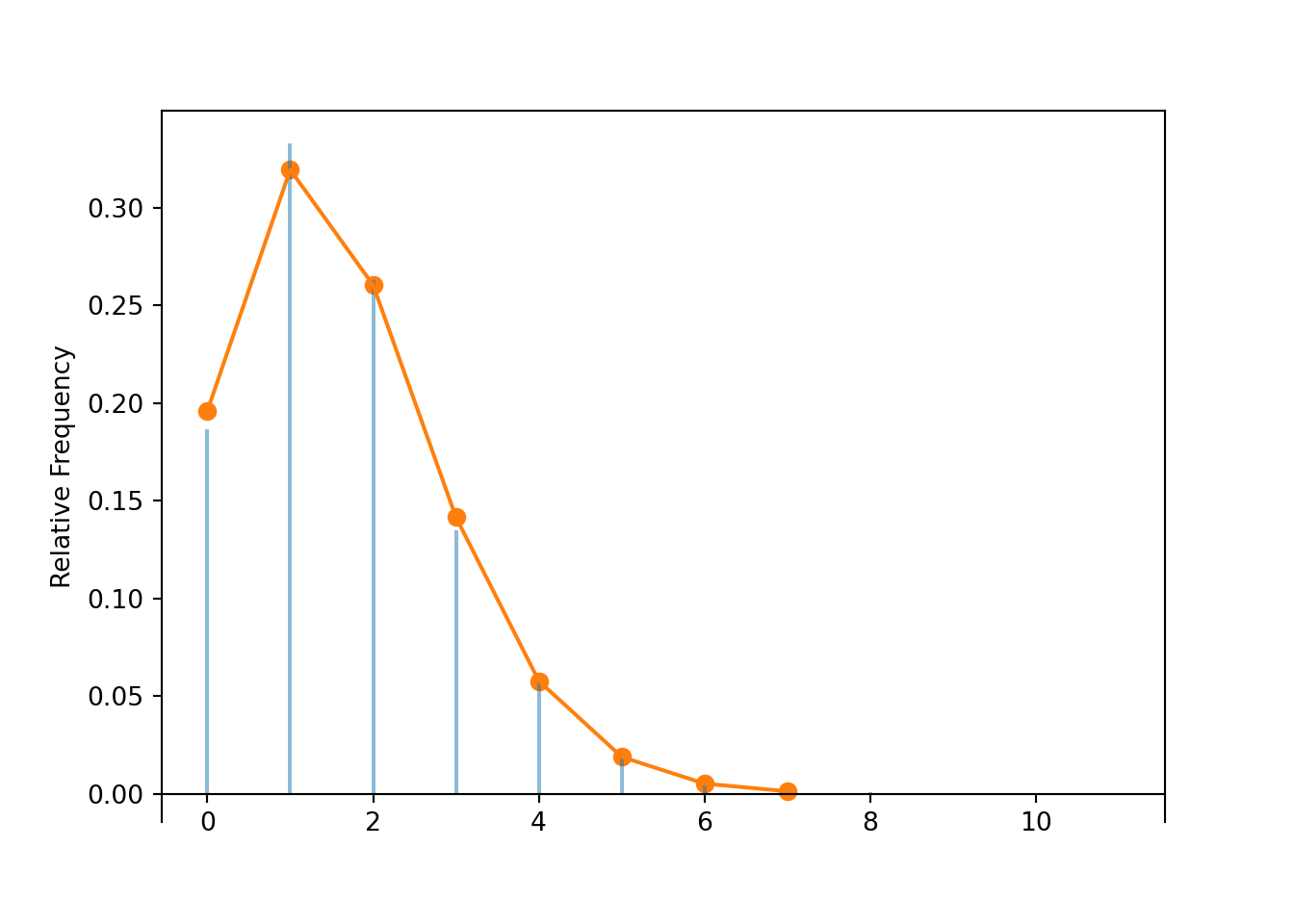

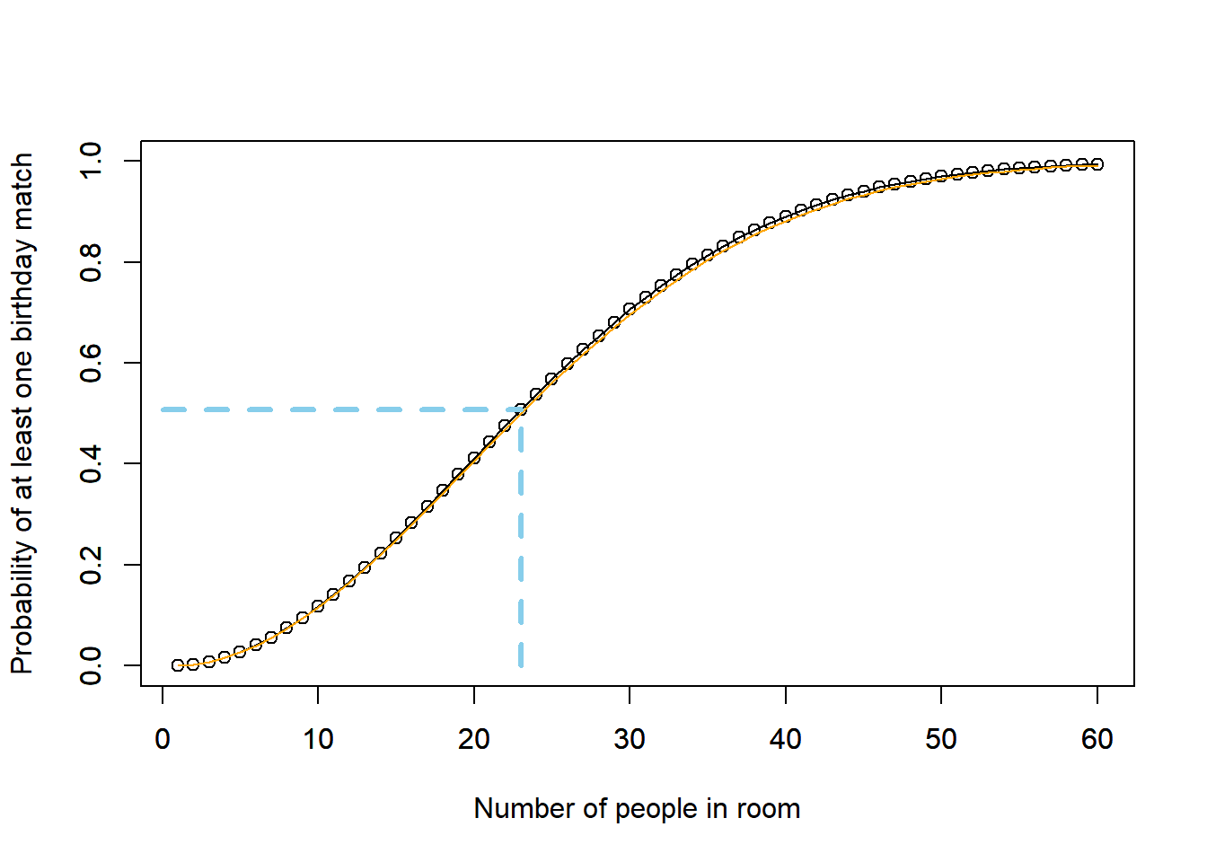
Loading

Sorry, something went wrong. Reload?

Sorry, we cannot display this file.

Sorry, this file is invalid so it cannot be displayed.

view raw poisson-birthdays.ipynb hosted with ❤ by GitHub

Figure 6.7: Probability of at least one birthday match as a function of the number of people in the room, along with the Poisson approximation. For 23 people, the probability of at least one birthday match is 0.507.

Poisson paradigm. Let $A_1, A_2, \ldots, A_n$ be a collection of $n$ events. Suppose event $i$ occurs with marginal probability $p_i=\textrm{P}(A_i)$. Let $N = \textrm{I}_{A_i} + \textrm{I}_{A_2} + \cdots + \textrm{I}_{A_n}$ be the random variable which counts the number of the events in the collection which occur. Suppose

• $n$ is “large”,
• $p_1, \ldots, p_n$ are “comparably small”, and
• the events $A_1, \ldots, A_n$ are “not too dependent”,

Then $N$ has an approximate Poisson distribution with parameter $\textrm{E}(N) = \sum_{i=1}^n p_i$.

We are leaving the terms “large”, “comparably small”, and “not too dependent” undefined. There are many different versions of Poisson approximations which make these ideas more precise. We only remark that Poisson approximation holds in a wide variety of situations.

The individual event probabilities $p_i$ can be different, but they must be “comparably small”. If one $p_i$ is much greater than the others, then the count random variable $N$ is dominated by whether event $A_i$ occurs or not. Also, as long as $\textrm{E}(N)$ is available, it is not necessary to know the individual $p_i$.

Even though $n$ is a constant in the above statement of the Poisson paradigm, there are other versions in which the number of events is random and unknown.

Example 6.22 Use Poisson approximation to approximate that probability that at least three people in a group of $n$ people share a birthday. How large does $n$ need to be for the probability to be greater than 0.5?

Show/hide solution

There are $\binom{n}{3}$ triples of people. We showed in Example 6.21 that the probability that any three people share a birthday is $\frac{1}{365^2}$. If $X$ is the number of triples that share a birthday, then $\textrm{E}(X) = \binom{n}{3}\left(\frac{1}{365^2}\right)$. The number of trials is large and the probability of success on any trial is small, so we assume $X$ has an approximate Poisson distribution. Therefore, the probability that at least three people share a birthday is $$1 - \textrm{P}(X=0) \approx 1-\exp\left(-\binom{n}{3}\left(\frac{1}{365^2}\right)\right)$$ The smallest $n$ for which this probability is greater than 0.5 is $n=84$. For $n\ge 124$, the probability is at least 0.9.

---

132. The parameter for a Poisson distribution is often denoted $\lambda$. However, we use $\mu$ to denote the parameter of a Poisson distribution, and reserve $\lambda$ to denote the rate parameter of a Poisson process (which has mean $\lambda t$ at time $t$).↩︎

133. There are easier proofs, e.g., using moment generating functions.↩︎

134. When there are $n$ trials, the probability of success on each of the $n$ trials is $p_n$. The subscript $n$ indicates that this value can change as $n$ changes (e.g. 1/10 when $n=10$, 1/100 when $n=100$), so that when $n$ is large $p$ is small enough to maintain relative “rarity”.↩︎