5.1 “Expected” value
Example 5.1 Recall the matching problem with \(n=4\): objects labeled 1, 2, 3, 4, are placed at random in spots labeled 1, 2, 3, 4, with spot 1 the correct spot for object 1, etc. Let the random variable \(X\) count the number of objects that are put back in the correct spot. Let \(\textrm{P}\) denote the probability measure corresponding to the assumption that the objects are equally likely to be placed in any spot, so that the 24 possible placements are equally.
In 3.20 we determined the distribution of \(X\), displayed in Table 5.1 below.
| x | P(X=x) |
|---|---|
| 0 | 0.3750 |
| 1 | 0.3333 |
| 2 | 0.2500 |
| 4 | 0.0417 |
- Describe two ways for simulating values of \(X\).
- The table below displays 10 simulated values of \(X\). How could you use the results of this simulation to approximate the long run average value of \(X\)? How could you get a better approximation of the long run average?
Table 5.2: Results of the number of matches (\(X\)) in 10 repetitions of the matching problem. Repetition Y 1 0 2 1 3 0 4 0 5 2 6 0 7 1 8 1 9 4 10 2 - Rather than adding the 10 values and dividing by 10, how could you simplify the calculation in the previous part?
- The table below summarizes 24000 simulated values of \(X\). Approximate the long run average value of \(X\).
Table 5.3: Results of the number of matches (\(X\)) in 24000 repetitions of the matching problem. Value of X Number of repetitions 0 8979 1 7993 2 6068 4 960 - Recall the distribution of \(X\). What would be the corresponding mathematical formula for the theoretical long run average value of \(X\)? This number is called the “expected value” of \(X\).
- Is the expected value the most likely value of \(X\)?
- Is the expected value of \(X\) the “value that we would expect” on a single repetition of the phenomenon?
- Explain in what sense the expected value is “expected”.
Solution. to Example 5.1
Show/hide solution
- We could shuffle cards labeled 1 through 4 and then distribute them into boxes labeled 1 through 4, and count the number of matches; that’s one simulated value of \(X\). Or we could construct a spinner corresponding to the distribution of \(X\) in the previous part and spin it once to obtain one simulated value of \(X\). We could then repeat either method many times to obtain many simulated values of \(X\).
- Compute the average of the 10 values simply by summing the values and dividing by 10. \[ \frac{0 + 1 + 0 + 0 + 2 + 0 + 1 + 1 + 4 + 2}{10} = 1.1 \] We could get a better approximation to the long run average value by simulating many values of \(X\) and then taking the average.
- Since every value of \(X\) is either 0, 1, 2, or 4, we can compute the sum of the simulated values by multiplying each possible value by the number of repetitions on which it occurs and then adding these terms. Then the average of the 10 values is equal to the sum of each possible value times its relative frequency \[ \frac{0 \times 4 + 1 \times 3 + 2 \times 2 + 4 \times 1}{10} = 0\left(\frac{4}{10}\right)+ 1\left(\frac{3}{10}\right) + 2\left(\frac{2}{10}\right)+ 4\left(\frac{1}{10}\right) = 1.1 \]
- Sum the 24000 values and divide by 24000. The only possible values of \(X\) are 0, 1, 2, 4 so the sum of simulated values, sorted, will be of the form \[ 0 + 0 + \cdots 0 + 1 + 1 + \cdots + 1 + 2 + 2 +\cdots + 2 + 4 + 4 + \cdots + 4. \] As in the previous part, since each of the 24000 values is either 0, 1, 2, or 4, the calculation of the sum can be simplified by multiplying each of the possible values by its frequency \[\begin{align*} & \qquad \frac{0 \times 8979 + 1 \times 7993 + 2 \times 6068 + 4 \times 960}{24000}\\ &= \frac{23969}{24000} = 0.99870\\ & = 0\left(\frac{8979}{24000}\right)+ 1\left(\frac{7993}{24000}\right) + 2\left(\frac{6068}{24000}\right)+ 4\left(\frac{960}{24000}\right) \end{align*}\] The average of the 24000 values is equal to the sum of each possible value times its simulated relative frequency. Based on the results of this simulation, the long run average value of \(X\) is approximately 0.9987.
- Theoretical probabilities are long run relative frequencies. In the long run, the simulated relative frequency of 0 will approach 9/24, of 1 will approach 8/24, etc. So in the long run, the calculation from the previous part should approach \[ 0\left(\frac{9}{24}\right)+ 1\left(\frac{8}{24}\right) + 2\left(\frac{6}{24}\right)+ 4\left(\frac{1}{24}\right) = 1 \] That is, we compute the probability-weighted average value. The expected value of \(X\) is 1.
- No, the most likely value of \(X\) is 0, not 1.
- No, 1 is not the value of \(X\) we would expect on a single repetition. The value 1 occurs with probability 1/3 and does not occur with probability 2/3. So it’s twice as likely to see a value other than 1 than to see 1. In particularly, 0 has a higher probability of occuring than 1.
- 1 is the value of \(X\) that would we expect to see on average in the long run. If the matching scenario were repeated many times, then the long run average number of matches would be (close to) 1.
The following Symbulate code simulates the matching problem. The main programming aspect is to write the count_matches function which takes as an input a sequence of prizes and returns as an output the number of matches. This function can then be used to define a RV (just as we use built in functions like sum and max). With Python’s zero-based indexing, the objects/spots are labeled 0, 1, 2, 3.
n = 4
labels = list(range(n)) # list of labels [0, ..., n-1]

# define a function which counts number of matches
def count_matches(x):
    count = 0
    for i in range(0, n, 1):
        if x[i] == labels[i]:
            count += 1
    return count

P = BoxModel(labels, size = n, replace = False)

X = RV(P, count_matches)

(RV(P) & X).sim(10)| Index | Result |
|---|---|
| 0 | ((0, 1, 2, 3), 4) |
| 1 | ((3, 1, 2, 0), 2) |
| 2 | ((1, 3, 2, 0), 1) |
| 3 | ((1, 3, 2, 0), 1) |
| 4 | ((2, 3, 1, 0), 0) |
| 5 | ((2, 1, 3, 0), 1) |
| 6 | ((0, 2, 1, 3), 2) |
| 7 | ((2, 3, 1, 0), 0) |
| 8 | ((0, 3, 1, 2), 1) |
| ... | ... |
| 9 | ((0, 3, 2, 1), 2) |
x = X.sim(24000)

x.tabulate()| Value | Frequency |
|---|---|
| 0 | 8975 |
| 1 | 8040 |
| 2 | 5998 |
| 4 | 987 |
| Total | 24000 |
x.plot()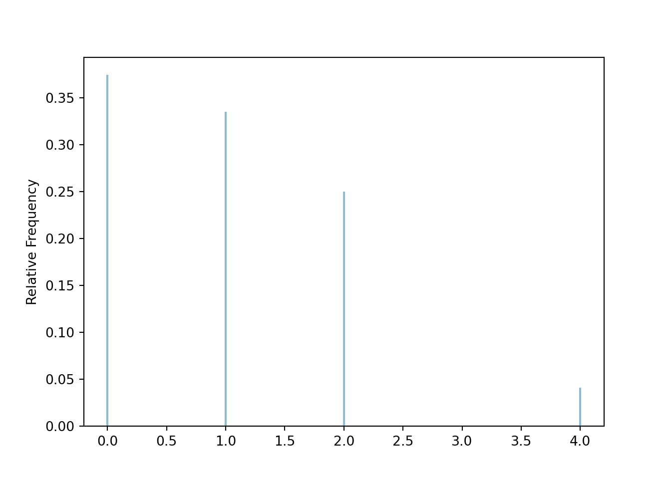
The average of the 24000 simulated values is founded by summing all the values and then by dividing by 24000, or just by using mean.
x.sum(), x.sum() / 24000, x.mean()## (23984, 0.9993333333333333, 0.9993333333333333)The previous example illustrates that the long run average value is also the probability-weighted average value. That is, we multiplied each value by its corresponding probability, determined by the pmf, and then summed. We can find the probability-weighted average value for continuous random variables analogously: multiply each possible value by its corresponding density, determined by the pdf, and then integrate.
Example 5.2 Let \(X\) be a random variable which has the Exponential(1) distribution. To motivate the computation of the expected value of a continuous random variable, we’ll first consider a discrete version of \(X\).
- How could you use simulation to approximate the long run average value of \(X\)?
- Suppose the values of \(X\) are truncated121 to integers. That is, 0.73 is recorded as 0, 1.15 is recorded as 1, 2.999 is recorded as 2, 3.001 is recorded as 3, etc. The following table summarizes 10000 simulated values of \(X\), truncated. Using just these values, how would you approximate the long run average value of \(X\)?
Table 5.4: 10000 simulated values of X, truncated, for X with an Exponential(1) distribution Truncated value of X Number of repetitions 0 6302 1 2327 2 915 3 287 4 94 5 43 6 22 7 5 8 4 9 1 - How could you approximate the probability that the truncated value of \(X\) is 0? 1? 2? Suggest a formula for the (approximate) long run average value of \(X\). (Don’t worry if the approximation isn’t great; we’ll see how to improve it.)
- Truncating to the nearest integer turns out not to yield a great approximation of the long run average value of \(X\). How could we get a better approximation?
- Suppose instead of truncating to an integer, we truncate to the first decimal. For example 0.73 is recorded as 0.7, 1.15 is recorded as 1.1, 2.999 is recorded as 2.9, 3.001 is recorded as 3.0, etc. Suggest a formula for the (approximate) long run average value of \(X\).
- We can continue in this way, truncating to the second decimal place, then the third, and so on. Considering what happens in the limit, suggest a formula for the theoretical long run average value of \(X\).
Solution. to Example 5.2
Show/hide solution
- Simulate many values of \(X\), e.g., using the Exponential(1) spinner, and average: sum the simulated values and divide by the number of simulated values. You can always approximate the long run average value of a random variable by simulating many values and averaging; it doesn’t matter if the random variable is discrete or continuous.
- The truncated random variable is a discrete random variable, so we can compute the average as in the matching problem \[ 0\left(\frac{6302}{10000}\right)+ 1\left(\frac{2327}{10000}\right)+2\left(\frac{915}{10000}\right) + 3\left(\frac{287}{10000}\right)+ \cdots + 9\left(\frac{1}{10000}\right) \]
- If \(X\) is between 0 and 1 then the truncated value is 1. We could find the probability that \(X\) is between 0 and 1 by integrating the pdf over this range. But we can approximate the probability by multiplying the pdf evaluated at 0.5 (the midpoint122) by the length of the (0, 1) interval: \(f(0.5)(1-0) = e^{-0.5}(1)\approx 0.607\). Recall the end of Section 4.3. Technically, the approximation is not great unless the interval is short, but it’s the idea that is important for now. Similarly the approximate probability that the truncated value is 1 is \(f(1.5)(2-1) = e^{-1.5}(1)\approx 0.223\), and the approximate probability that the truncated value is 2 is \(f(2.5)(3-2) = e^{-2.5}(1)\approx 0.082\). Following this pattern, a reasonable formula for the (approximate) long run average value of \(X\) seems to be \[\begin{align*} & \qquad 0\left(f(0+ 0.5)(1)\right)+ 1\left(f(1 + 0.5)(1)\right)+2\left(f(2+0.5)(1)\right) + 3\left(f(3 + 0.5)(1)\right) + \cdots \\ & = \sum_{x=0}^\infty x f(x + 0.5) (1)\\ & = \sum_{x=0}^\infty x e^{-(x + 0.5)} (1) \end{align*}\] where the sum is over values \(x = 0, 1, 2, \ldots\). Plugging in \(f(x + 0.5) = e^{-(x+0.5)}\) to the above yields 0.558. (This is a bad approximation, but the following parts refine it. Using the left endpoint instead of the midpoint, that is, replacing \(f(x)=e^{-x}\) instead of \(f(x+0.5)=e^{-(x+0.5)}\), yields 0.92.)
- Rather than truncating to integers, truncate to the first decimal, or the second, or the third. Or better yet don’t truncate; \(X\) is continuous after all. But it helps to consider what would happen if \(X\) were discrete first.
- Now the possible values would be 0, 0.1, 0.2, etc. The truncated value would be 0 if \(X\) lies in the interval (0, 0.1). We could approximate this probability with \(f(0.05)(0.1-0) = e^{-0.05}(0.1)\). We could approximate the probability that \(X\) lies in the interval (0.1, 0.2), so the truncated value is 0.1, with \(f(0.15)(0.2-0.1) = e^{-0.15}(0.1)\). Following this pattern, a reasonable formula for the (approximate) long run average value of \(X\) seems to be \[\begin{align*} & \qquad 0\left(f(0+ 0.05)(0.1)\right)+ 0.1\left(f(0.1 + 0.05)(0.1)\right)+0.2\left(f(0.2+0.05)(0.1)\right) + 0.3\left(f(0.3 + 0.05)(0.1)\right) + \cdots \\ & = \sum_{x=0}^\infty x f(x + 0.05) (0.1)\\ & = \sum_{x=0}^\infty x e^{-(x + 0.05)} (0.1) \end{align*}\] where the sum is over values \(x = 0, 0.1, 0.2, \ldots\). Plugging in \(f(x + 0.5) = e^{-(x+0.5)}\) to the above yields 0.950.
- Truncating to the second decimal place suggests a formula for the long run average of
\[\begin{align*}
& \qquad 0\left(f(0+ 0.005)(0.01)\right)+ 0.01\left(f(0.01 + 0.005)(0.01)\right)+0.02\left(f(0.02+0.005)(0.01)\right) + 0.03\left(f(0.03 + 0.005)(0.01)\right) + \cdots
\\
& = \sum_{x=0}^\infty x f(x + 0.005) (0.01)\\
& = \sum_{x=0}^\infty x e^{-(x + 0.005)} (0.01)
\end{align*}\]
where the sum is over values \(x = 0, 0.01, 0.02, \ldots\). Plugging in \(f(x) = e^{-x}\) to the above yields 0.995.
If \(\Delta x\) represents the level of truncation, e.g., \(\Delta x = 0.01\) for truncating to the second decimal place, then a general formula is \[\begin{align*} & \qquad \sum_{x=0}^\infty x f(x + \Delta x / 2) \Delta x\\ & = \sum_{x=0}^\infty x e^{-x + \Delta x / 2} \Delta x\\ & \approx \sum_{x=0}^\infty x e^{-x} \Delta x \end{align*}\] In the limit as \(\Delta x\) approaches 0, \(f(x + \Delta x /2)\) approaches \(f(x)=e^{-x}\), there are more and more terms in the sum, and the sum approaches an integral over \(x\) values, \[\begin{align*} & \qquad \int_0^\infty x f(x) dx\\ & = \int_0^\infty x e^{-x} dx \end{align*}\]
Definition 5.1 The expected value (a.k.a. expectation a.k.a. mean), of a random variable \(X\) defined on a probability space with measure \(\textrm{P}\), is a number denoted \(\textrm{E}(X)\) representing the probability-weighted average value of \(X\). Expected value is defined as
\[\begin{align*} & \text{Discrete $X$ with pmf $p_X$:} & \textrm{E}(X) & = \sum_x x p_X(x)\\ & \text{Continuous $X$ with pdf $f_X$:} & \textrm{E}(X) & =\int_{-\infty}^\infty x f_X(x) dx \end{align*}\]
Note well that \(\textrm{E}(X)\) represents a single number.
For a discrete random variable, the sum is over all possible values of \(X\), that is, values of \(x\) with \(p_X(x)>0\). For a continuous random variable, the generic bounds \((-\infty, \infty)\) should be replaced with the possible values of \(X\); that is, the bounds correspond to intervals of \(X\) with \(f_X(x)>0\).
Example 5.3 Let \(X\) be a random variable which has the Exponential(1) distribution.
- Donny Dont says \(\textrm{E}(X) = \int_0^\infty e^{-x}dx = 1\). Do you agree?
- Compute \(\textrm{E}(X)\).
- Compute \(\textrm{P}(X = \textrm{E}(X))\).
- Compute \(\textrm{P}(X \le \textrm{E}(X))\).
- Find the median value of \(X\). Is the median less than, greater than, or equal to the mean? Why does this make sense?
Solution. to Example 5.3
Show/hide solution
- Donny happened to get the correct value, but that’s just coincidence. His method is wrong. Donny integrated \(\int_{-\infty}^\infty f_X(x)dx\) which will always be 1. To get the expected value, you need to find the probability weighted average value of \(x\): \(\int_{-\infty}^\infty x f_X(x)dx\). Forgetting the \(x\) is a common mistake. Don’t forget the \(x\).
- Since \(X\) is continuous, with pdf \(f_X(x) = e^{-x}, x > 0\), we integrate123 \[ \textrm{E}(X) = \int_0^\infty x e^{-x}dx = 1 \] Notice that the bounds of the integral correspond to the interval of possible values of \(X\).
- The notation \(\textrm{P}(X = \textrm{E}(X))\) might seem strange at first. But keep in mind that \(\textrm{E}(X)\) is a single number, so \(\textrm{P}(X = \textrm{E}(X))\) makes as much sense as \(\textrm{P}(X = 1)\). Since \(X\) is a continuous random variable, the probability that it equals any particular number is 0.
- We can use the cdf of \(X\): \(\textrm{P}(X \le \textrm{E}(X))=\textrm{P}(X \le 1)=F_X(1) = 1-e^{-1}\approx0.632\).
- The previous part shows that 1 is the 63rd percentile, so we know the mean of 1 will be greater than the median. The cdf is \(1-e^{-x}\), so setting the cdf to 0.5 and solving for \(x\) yields the median: \(0.5=1-e^{-x}\) implies \(x=-\log(1-0.5)\approx 0.693\). The mean is greater than the median because the large values in the right tail “pull the average up”.
X = RV(Exponential(1))

x = X.sim(10000)

x| Index | Result |
|---|---|
| 0 | 0.27052598475824624 |
| 1 | 2.470866623870595 |
| 2 | 0.6731067391331644 |
| 3 | 1.5711848806200863 |
| 4 | 4.91057385015532 |
| 5 | 0.5906457388971905 |
| 6 | 0.8729712429177028 |
| 7 | 2.21373783616862 |
| 8 | 1.7553848970561459 |
| ... | ... |
| 9999 | 0.2601169061562036 |
x.sum(), x.sum() / 10000, x.mean()## (10152.352736413914, 1.0152352736413914, 1.0152352736413914)The expected value is the “balance point” (center of gravity) of a distribution. Imagine the impulse plot/histogram is constructed by stacking blocks on a board. Then \(\textrm{E}(X)\) represents where you would need to place a stand underneath the board so that it doesn’t tip to one side.
The probability of an event \(A\), \(\textrm{P}(A)\), is defined by the underlying probability measure \(\textrm{P}\). However, \(\textrm{P}(A)\) can be interpreted as a long run relative frequency and can be approximated via a simulation consisting of many repetitions of the random phenomenon. Similarly, the expected value of a random variable \(X\) is defined by the probability-weighted average according to the underlying probability measure. But the expected value can also be interpreted as the long-run average value, and so can be approximated via simulation. The fact that the long run average is equal to the probability-weighted average is known as the law of large numbers. (We will see the law of large numbers in more detail later.)
Recall the discussion in Section 2.9.1, which we briefly recap here in the context of the matching problem.
The plots below illustrates the running average of \(X\) in Example 5.1.
| Repetition | Value of X | Running average of X |
|---|---|---|
| 1 | 0 | 0.000 |
| 2 | 1 | 0.500 |
| 3 | 0 | 0.333 |
| 4 | 0 | 0.250 |
| 5 | 2 | 0.600 |
| 6 | 0 | 0.500 |
| 7 | 1 | 0.571 |
| 8 | 1 | 0.625 |
| 9 | 4 | 1.000 |
| 10 | 2 | 1.100 |
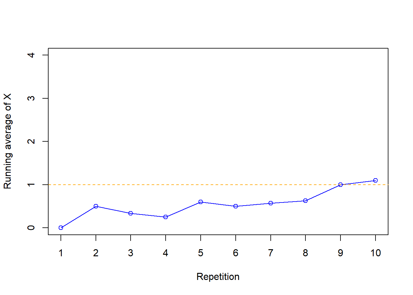
Figure 5.1: Running average for number of matches in the matching problem based on the simulation results in Table 5.2.
As the number of repetitions increases, the running average of the number of matches tends to stabilize around the expected value of 1, regardless of the particular sequence of \(X\) values in the simulation. There is some natural simulation variability in the running average, but that variability decreases as the number of independently simulated values used to compute the average increases.
rmax = 100

P = BoxModel([0, 1, 2, 4], probs = [9/24, 8/24, 6/24, 1/24]) ** rmax

X = RV(P)

Xbar_r = RandomProcess(P)

for r in range(rmax):
    Xbar_r[r] = X[0:(r + 1)].apply(mean)

Xbar_r.sim(5).plot(tmax = rmax)

plt.ylim(0, 4);
plt.xlabel('Repetition');
plt.ylabel('Running average of X');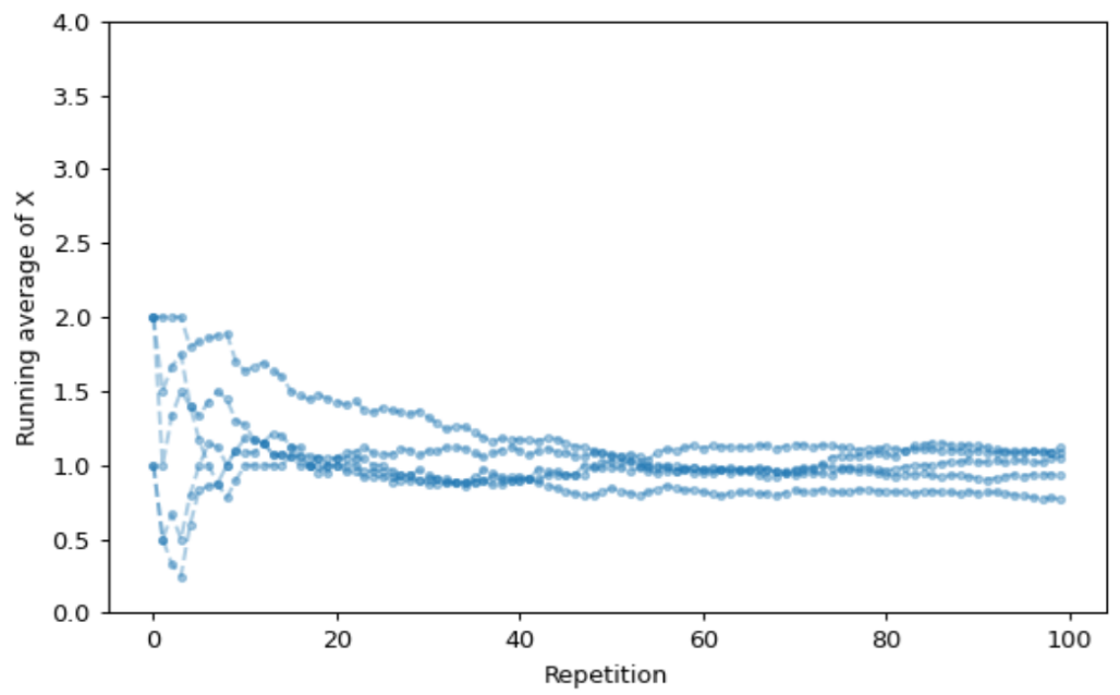
Figure 5.2: An illustration of the law of large numbers for the matching problem with \(n=4\). The plot displays the running average of simulated values of \(X\), the number of matches, as the number of simulated values increases (from 1 to 100) for each of five separate simulations. We can see that when the number of simulated values is small, the averages vary a great deal from simulation to simulation. But as the number of simulated values increases, the average for each simulation starts to settle down to 1, the theoretical expected value.
An expected value is defined as a probability-weight average value, but it often helps to interpret expected value as a long run average value. From a simulation perspective, you can read the symbol \(\textrm{E}(\cdot)\) as
- Simulate lots of values of what’s inside \((\cdot)\)
- Compute the average. This is a “usual” average; just sum all the simulated values and divide by the number of simulated values.
Example 5.4 Consider the probability space corresponding to a sequence of three flips of a fair coin. Let \(X\) be the number of H, \(Y\) the number of tails, and \(Z\) the length of the longest streak of H in a row (which can be 0 (TTT), 1 (e.g., HTT), 2 (e.g. THH), or 3 (HHH)).
- Compute \(\textrm{E}(X)\).
- Find and interpret \(\textrm{P}(X=\textrm{E}(X))\).
- Is \(\textrm{E}(X)\) the “value that we would expect” on a single repetition of the process?
- Write a clearly worded sentence interpreting \(\textrm{E}(X)\) in context.
- Here is Donny Dont’s response to the previous part: “1.5 is the long run average value.” Does he get full credit? If not, what is wrong/missing?
- Donny tries again: “1.5 is the average number of heads in three flips.” Does he get full credit? If not, what is wrong/missing?
- Donny tries yet again: “If a coin is flipped three times and the number of heads is recorded and this process is repeated many times, then the number of heads is close to 1.5 in the long run.” Does he get full credit? If not, what is wrong/missing?
- Without doing any calculations, find \(\textrm{E}(Y)\). Explain.
- Without doing any calculations determine if \(\textrm{E}(Z)\) will be greater than, less than, or equal to \(\textrm{E}(X)\). Confirm your guess by computing \(\textrm{E}(Z)\).
- Suppose now that the coin is biased and has a probability of 0.6 of landing on heads. Without doing any calculations: Would \(\textrm{E}(X)\) change? Would \(\textrm{E}(X)\) be equal to \(\textrm{E}(Y)\)?
Solution. to Example 5.4
Show/hide solution
- \(X\) has a Binomial(3, 0.5) distribution, taking values 0, 1, 2, 3, with respective probability 1/8, 3/8, 3/8, 1/8. \[ \textrm{E}(X)=0(1/8) + 1(3/8) + 2(3/8) + 3(1/8) = 1.5. \]
- \(\textrm{P}(X=\textrm{E}(X))=\textrm{P}(X = 1.5) = 0\). Remember, \(\textrm{E}(X)\) is just a number.
- \(E(X)\) is not the “value that we would expect” on a single repetition of the process; it’s not even possible to observe an \(X\) of 1.5 on a single repetition. You can’t flip a coin 3 times and observe 1.5 heads in the 3 flips.
- Over many sets of 3 fair coin flips, we expect 1.5 heads per set on average in the long run.
- Donny only gets partial credit; he’s missing the context. The long run average value of what?
- Donny only gets partial credit; he’s missing any reference to the long run.
- Donny only gets partial credit. His sentence is pretty good with reference to the context and a long run description. But he’s missing one extremely important word: average.
- If the coin is fair then \(X\) and \(Y\) have the same distribution and so \(\textrm{E}(Y) =\textrm{E}(X) = 1.5\). If \(X\) and \(Y\) have the same long run pattern of variability, then they will have the same long run average value.
- For any outcome, the length of the longest streak of H can’t be more than the number of H. That is \(X\ge Z\), so we must have \(\textrm{E}(X) \ge \textrm{E}(Z)\). If for every outcome \(X\) is at least as large as \(Z\), then the long run average value of \(X\) should be at least as large as the long run average value of \(Z\). See Table 3.1. \(\textrm{E}(Z)=0(1/8) + 1(4/8) + 2(2/8) + 3(1/8) = 11/8=1.375\).
- The sample space and the RVs would not change. But the probability measure \(\textrm{P}\) would change and so would the distribution of \(X\) and \(\textrm{E}(X)\). Also, the distribution of \(X\) and \(Y\) would not be the same anymore, and neither would the expected values.
| Outcome | X | Y | Z |
|---|---|---|---|
| HHH | 3 | 0 | 3 |
| HHT | 2 | 1 | 2 |
| HTH | 2 | 1 | 1 |
| THH | 2 | 1 | 2 |
| HTT | 1 | 2 | 1 |
| THT | 1 | 2 | 1 |
| TTH | 1 | 2 | 1 |
| TTT | 0 | 3 | 0 |
If two random variables \(X\) and \(Y\) have the same distribution (i.e., same long run pattern of variation) then they have the same expected value (i.e., same long run average value).
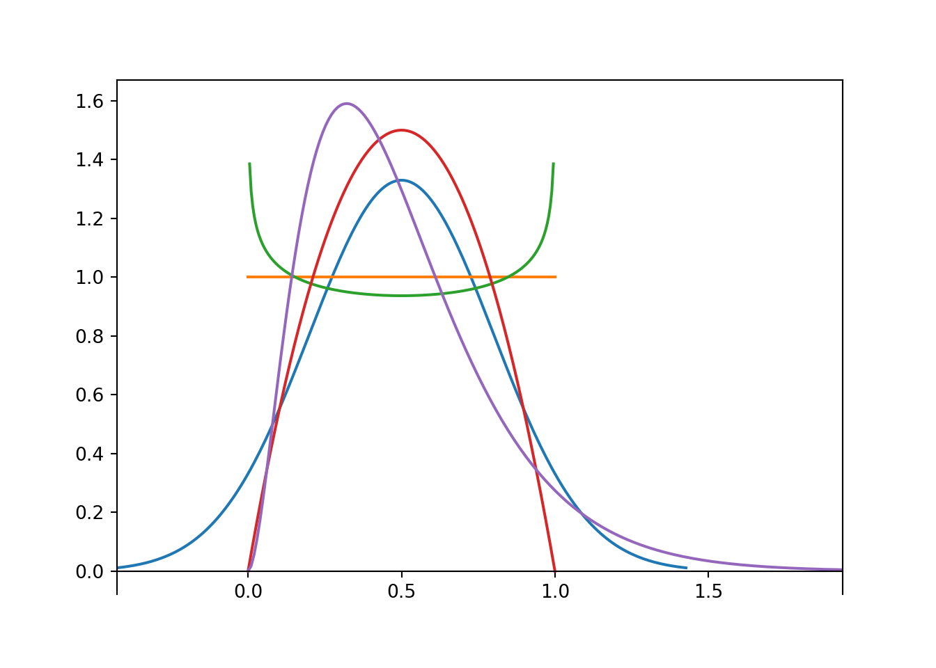
But the converse is not true: \(\textrm{E}(X) = \textrm{E}(Y)\) does NOT imply that \(X\) and \(Y\) have the same distribution. For example, the random variables in Example 5.1 and Example 5.3 both have expected value 1, but they are two very different random variables. Expected value is just one summary characteristic of a distribution, i.e., the average. But there can be much more to the pattern of variation, i.e., the distribution. The following plot illustrates just a few different distributions that all have expected value 0.5. (Don’t worry about what these distributions are for now; we’ll encounter some of them later. Just know that they represent different patterns of variability.)
If \(X\le Y\) — that is, if \(X(\omega)\le Y(\omega)\) for all124 \(\omega\in\Omega\) — then \(\textrm{E}(X)\le\textrm{E}(Y)\). That is, if for every outcome the value of \(X\) is no bigger than the value of \(Y\), then the long run average value of \(X\) can’t be any bigger than the long run average value of \(Y\).
The distribution of a RV and its expected value depend on the probability measure \(\textrm{P}\). If the probability measure changes (e.g., from representing a fair coin to a biased coin) then distributions and expected values of RVs will change. Remember that \(\textrm{P}\) represents a probability measure that incorporates all the underlying assumptions about the random phenomenon (the symbol \(\textrm{P}\) is more than just shorthand for “probability”). In the same way, the symbol \(\textrm{E}\) is more than just shorthand for “expected value”. Rather \(\textrm{E}\) represents the probability-weighted/long run average value according to all the underlying assumptions of the random phenonemon as specified by the probability measure \(\textrm{P}\). In fact, a more appropriate symbol might be \(\textrm{E}_{\textrm{P}}\) to emphasize the dependence on the probability measure. We will only use such notation if multiple probability measures are being considered on the same sample space, e.g., \(\textrm{E}_{\textrm{P}}\) represents the expected value according to probability measure \(\textrm{P}\) (e.g., fair coin), while \(\textrm{E}_{\textrm{Q}}\) represents expected value according to probability measure \(\textrm{Q}\) (e.g., biased coin).
Example 5.5 Recall Example 4.7 in which we assume that \(X\), the number of home runs hit (in total by both teams) in a randomly selected Major League Baseball game, has a Poisson(2.3) distribution with pmf
\[ p_X(x) = \begin{cases} e^{-2.3} \frac{2.3^x}{x!}, & x = 0, 1, 2, \ldots\\ 0, & \text{otherwise.} \end{cases} \]
- Recall from Example 4.7 that \(\textrm{P}(X \le 13) =0.9999998\). Evaluate the pmf for \(x=0, 1, \ldots, 13\) and use arithmetic to compute \(\textrm{E}(X)\). (This will technically only give an approximation, since there is non-zero probability that \(X>13\), but the calculation will give you a concrete example before jumping to the next part.)
- Use the pmf and infinite series to compute \(\textrm{E}(X)\).
- Interpret \(\textrm{E}(X)\) in context.
Solution. to Example 5.5
See Example 4.7 and the discussion following it for calculation of the probabilities. \[ {\scriptsize (0)(0.10026)+(1)(0.2306)+(2)(0.26518)+(3)(0.20331)+(4)(0.1169)+(5)(0.05378)+(6)(0.02061)+(7)(0.00677)+(8)(0.00195)+(9)(0.0005)+(10)(0.00011)+(11)(0.00002)+(12)(0)+(13)(0) = 2.3 } \]
\(X\) is a discrete random variable that takes infinitely many possible values. The sum in the expected value definition is now an infinite series.
\[\begin{align*} \textrm{E}(X) & = \sum_{x = 0}^\infty x p_X(x) & & \\ & = \sum_{x = 0}^\infty x \left(e^{-2.3} \frac{2.3^x}{x!}\right) & & \\ & = \sum_{x = 1}^\infty e^{-2.3} \frac{2.3^x}{(x-1)!}& & (x=0 \text{ term is 0})\\ & = 2.3 \sum_{x = 1}^\infty e^{-2.3} \frac{2.3^{x-1}}{(x-1)!} & & \\ & = 2.3(1) & & \text{Taylor series for $e^u$ at $u=2.3$} \end{align*}\]
So \(\textrm{E}(X)=2.3\).
Over many MLB games, there are 2.3 home runs hit per game on average in the long run. Note that 2.3 is the observed average number of home runs per game in the 2018 MLB season data, displayed in Figure 4.6.
In general, if \(X\) has a Poisson(\(\mu\)) distribution, then \(\textrm{E}(X)=\mu\).
Example 5.6 Let \(X\) be a random variable with a Uniform(0, 1) distribution. Compute \(\textrm{E}(X)\). Then suggest a general formula for the expected value of a random variable with a Uniform(\(a\), \(b\)) distribution.
Solution. to Example 5.6
Show/hide solution
Since the expected value is the balance point, it seems that the expected value for a Uniform distribution should just be the midpoint of the interval of possible values.
For Uniform(0, 1), the pdf is a constant of 1 between 0 and 1.
\[ \textrm{E}(X) = \int_0^1 x \left(1\right) dx = x^2/2 \Bigg|_{0}^{1} = \frac{1}{2} \]
For Uniform(\(a\), \(b\)) the pdf is a constant of \(\frac{1}{b-a}\) between \(a\) and \(b\).
\[ \textrm{E}(X) = \int_a^b x \left(\frac{1}{b-a}\right) dx = \frac{1}{2(b-a)} x^2 \Bigg|_{a}^{b} = \frac{b^2 - a^2}{2(b-a)} = \frac{a+b}{2} \]
Recall that the indicator random variable corresponding to event \(A\) is defined as \[ \textrm{I}_A(\omega) = \begin{cases} 1, & \omega \in A,\\ 0, & \omega \notin A \end{cases} \]
Indicators provide the bridge between events (sets) and random variables (functions), and between probabilities (of events) and expected values (of random variables).
\[ \textrm{E}\left(\textrm{I}_A\right) = \textrm{P}(A) \]
We could also round to the nearest integer. Whether we truncate or round won’t matter as we consider what happens in the limit.↩︎
In the limit, any value in (0, 1) would work. We use the midpoint mostly because just using using 0 results in an approximate probability of \(e^{-0}(1)=1\), an egregious approximation of the true probability \(1-e^{-1}\approx 0.632\)↩︎
If you really wanted to, you could compute this integral using integration by parts.↩︎
This is sufficient, but technically not necessary. If \(X\le Y\) almost surely — that is, if \(\textrm{P}(X\le Y)=1\) — then \(\textrm{E}(X)\le \textrm{E}(Y)\).↩︎