5.4 Covariance and correlation
Quantities like expected value and variance summarize characteristics of the marginal distribution of a single random variable. When there are multiple random variables their joint distribution is of interest. Covariance summarizes in a single number a characteristic of the joint distribution of two random variables, namely, the degree to which they “co-deviate from the their respective means”.
Recall Section 2.12 where we saw that covariance of random variables \(X\) and \(Y\) is the long run average of the product of the paired deviations from the respective means
\[ \text{Covariance($X$, $Y$)} = \text{Average of} ((X - \text{Average of }X)(Y - \text{Average of }Y)) \] It turns out that covariance is equivalent to the average of the product minus the product of the averages.
\[ \text{Covariance($X$, $Y$)} = \text{Average of} XY - (\text{Average of }X)(\text{Average of }Y) \]
Translating the long run averages into expected values yields the following definition.
Definition 5.5 The covariance between two random variables \(X\) and \(Y\) is \[\begin{align*} \textrm{Cov}(X,Y) & = \textrm{E}\left[\left(X-\textrm{E}[X]\right)\left(Y-\textrm{E}[Y]\right)\right]\\ & = \textrm{E}(XY) - \textrm{E}(X)\textrm{E}(Y) \end{align*}\]
The first line above defines covariance as the long run average product of paired deviations from the mean. The second provides an equivalent formula that simplifies computation. Namely, covariance is the expected value of the product minus the product of expected values. (Remember that in general \(\textrm{E}(XY)\) is not equal to \(\textrm{E}(X)\textrm{E}(Y)\).)
Example 5.21 Consider the probability space corresponding to two rolls of a fair four-sided die. Let \(X\) be the sum of the two rolls, \(Y\) the larger of the two rolls, \(W\) the number of rolls equal to 4, and \(Z\) the number of rolls equal to 1.
- Specify the joint pmf of \(X\) and \(Y\). (These first few parts are review of things we have covered before.)
- Find the marginal pmf of \(X\) and \(\textrm{E}(X)\).
- Find the marginal pmf of \(Y\) and \(\textrm{E}(Y)\).
- Find \(\textrm{E}(XY)\). Is it equal to \(\textrm{E}(X)\textrm{E}(Y)\)?
- Find \(\textrm{Cov}(X, Y)\). Why is the covariance positive?
- Is \(\textrm{Cov}(X, W)\) positive, negative, or zero? Why?
- Is \(\textrm{Cov}(X, Z)\) positive, negative, or zero? Why?
- Let \(V=W+Z\). Is \(\textrm{Cov}(X, V)\) positive, negative, or zero? Why?
- Is \(\textrm{Cov}(W, Z)\) positive, negative, or zero? Why?
Solution. to Example 5.21
Show/hide solution
- See Example 2.23 for the joint and marginal distributions.
- \(\textrm{E}(X)= 5\).
- \(\textrm{E}(Y) = 1(1/16) + 2(3/16) + 3(5/16) + 4(7/16) = 3.125\).
- \(\textrm{E}(XY)=(2)(1)(1/16) + (3)(2)(2/16) + \cdots (8)(4)(1/16) = 16.875\). This is not equal to \(\textrm{E}(X)\textrm{E}(Y) = (5)(3.125) = 15.625.\)
- \(\textrm{Cov}(X, Y) = \textrm{E}(XY) - \textrm{E}(X)\textrm{E}(Y) = 16.875 - 15.625 = 1.25.\) There is an overall positive association; above average values of \(X\) tend to be associated with above average values of \(Y\) (e.g., (7, 4), (8, 4)), and below average values of \(X\) tend to be associated with below average values of \(Y\) (e.g., (2, 1), (3, 2)).
- \(\textrm{Cov}(X, W)>0\). If \(W\) is large (roll many 4s) then \(X\) (sum) tends to be large.
- \(\textrm{Cov}(X, Z)<0\). If \(Z\) is large (roll many 1s) then \(X\) (sum) tends to be small.
- \(\textrm{Cov}(X, W + Z)=0\). Basically, the positive association between \(X\) and \(W\) cancels out with the negative association of \(X\) and \(Z\). \(V\) is large when there are many 1s or many 4s, or some mixture of 1s and 4s. So knowing that W is large doesn’t really tell you anything about the sum.
- \(\textrm{Cov}(W, Z)<0\). There is a fixed number of rolls. If you roll lots of 4s (\(W\) is large) then there must be few rolls of 1s (\(Z\) is small).
The sign of the covariance indicates the overall direction of the association between \(X\) and \(Y\).
- \(\textrm{Cov}(X,Y)>0\) (positive association): above average values of \(X\) tend to be associated with above average values of \(Y\)
- \(\textrm{Cov}(X,Y)<0\) (negative association): above average values of \(X\) tend to be associated with below average values of \(Y\)
- \(\textrm{Cov}(X,Y)=0\) indicates that the random variables are uncorrelated: there is no overall positive or negative association. But be careful: if \(X\) and \(Y\) are uncorrelated there can still be a relationship between \(X\) and \(Y\); there is just no overall positive or negative association.. We will see examples that demonstrate that being uncorrelated does not necessarily imply that random variables are independent.
Example 5.22 In Example 2.57, how could we use simulation to approximate \(\textrm{Cov}(X, Y)\)? Donny Dont’s Symbulate code is below. Explain to Donny in words the correct simulation process, and why his code does not reflect that process. What is the correct code?
P = DiscreteUniform(1, 4) ** 2
X = RV(P, sum)
Y = RV(P, max)

x = X.sim(10000)
y = Y.sim(10000)

(x * y).mean() - x.mean() * y.mean()Solution. to Example 5.22
Show/hide solution
Donny’s code attempts to simulate values of \(X\) and values of \(Y\) separately, from each of their marginal distributions. However, to approximate the covariance we need to simulate \((X, Y)\) pairs from the joint distribution. See the code below. (Otherwise, Donny’s code is fine.)
Since \(\textrm{Cov}(X, Y)\) is based on expected values, it can be approximated by simulating appropriate long run averages.
- Simulate an \((X, Y)\) pair from the joint distribution.
- Find the value of the product \(XY\) for the simulated pair.
- Repeat many times, simulating many \((X, Y)\) pairs and finding their product \(XY\).
- Average the simulated values of the product \(XY\) to approximate \(\textrm{E}(XY)\).
- Average the simulated values of \(X\) to approximate \(\textrm{E}(X)\).
- Average the simulated values of \(Y\) to approximate \(\textrm{E}(Y)\).
- \(\textrm{Cov}(X, Y)\) is approximately the average of the product minus the product of the averages.
The following code illustrates how to approximate covariance via simulation in the context of the previous example. The key is to first simulate \((X, Y)\) pairs with the proper joint distribution.
P = DiscreteUniform(1, 4) ** 2
X = RV(P, sum)
Y = RV(P, max)

xy = (X & Y).sim(10000)

xy| Index | Result |
|---|---|
| 0 | (3, 2) |
| 1 | (2, 1) |
| 2 | (6, 3) |
| 3 | (6, 4) |
| 4 | (6, 4) |
| 5 | (4, 3) |
| 6 | (4, 3) |
| 7 | (7, 4) |
| 8 | (7, 4) |
| ... | ... |
| 9999 | (4, 3) |
plt.figure()
xy.plot('tile')
plt.show()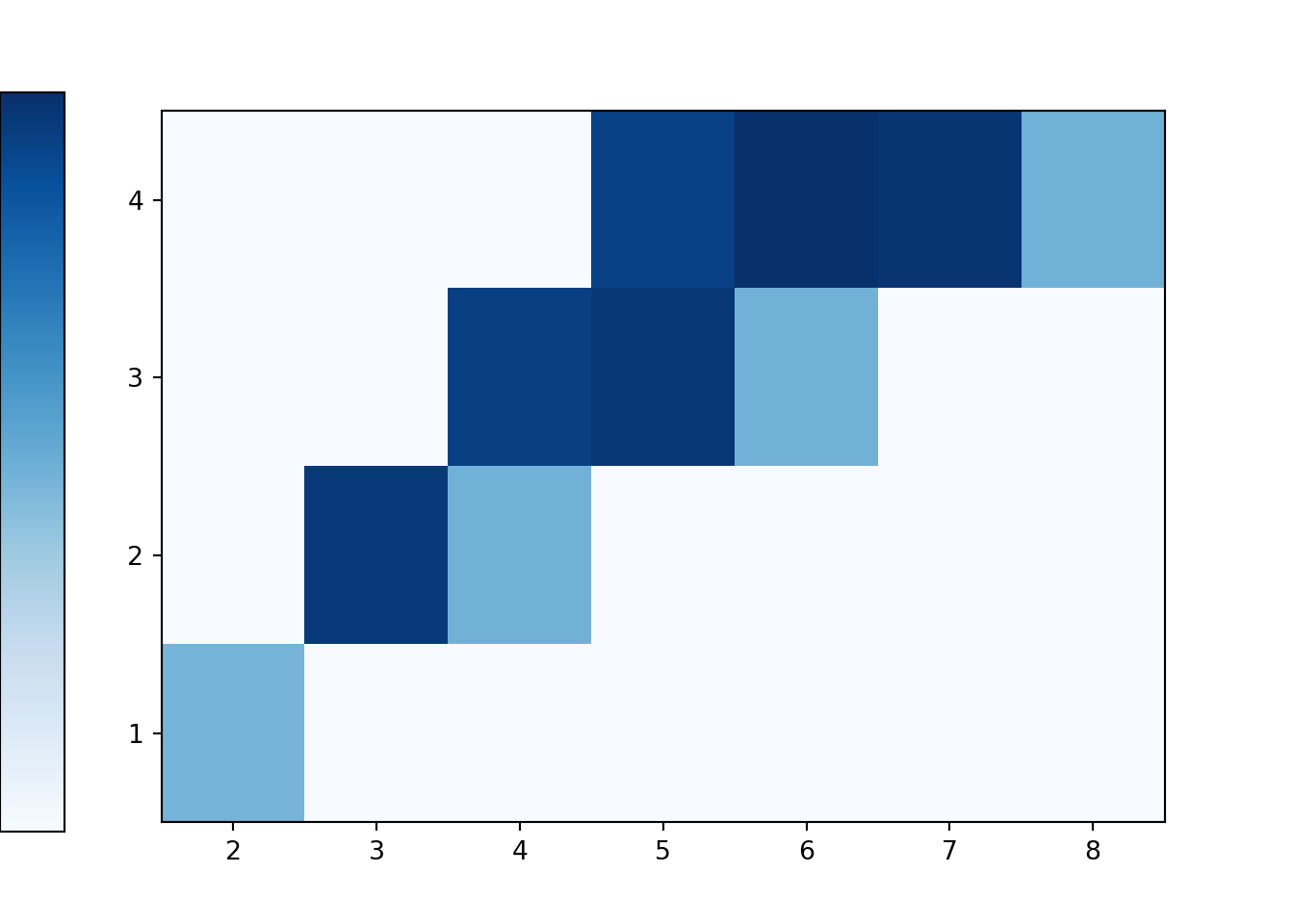
The simulated \((X, Y)\) pairs are stored as xy, a matrix with two columns (one for \(X\) and one for \(Y\)) and a row for each repetition of the simulation. The simulated \(X\) values in the first column of xy can be extracted with x = xy[0]. (Remember Python’s zero-based indexing.) The simulated \(Y\) values in the second column of xy can be extracted with y = xy[1]. The product x * y will multiply \(XY\) for each simulated \((X, Y)\) pair, row by row.
x = xy[0]
y = xy[1]

x * y| Index | Result |
|---|---|
| 0 | 6 |
| 1 | 2 |
| 2 | 18 |
| 3 | 24 |
| 4 | 24 |
| 5 | 12 |
| 6 | 12 |
| 7 | 28 |
| 8 | 28 |
| ... | ... |
| 9999 | 12 |
We can then approximate the covariance with the average of the product minus the product of the averages.
(x * y).mean() - x.mean() * y.mean()## 1.2525323400000001The .cov() command performs the above calculation.
xy.cov()## 1.2525323399999988Example 5.23 Recall Example ??. Spin the Uniform(1, 4) spinner twice and let \(X\) be the sum and \(Y\) the larger of the two spins. Sketch a plot of the joint distribution; is \(\textrm{Cov}(X, Y)\) positive, negative, or zero? Then use simulation to approximate the covariance.
Show/hide solution
Covariance is positive as above average values of \(X\) tend to be associated with above average values of \(Y\). Simulation show the covariance is about 0.75.
P = Uniform(1, 4) ** 2
X = RV(P, sum)
Y = RV(P, max)

xy = (X & Y).sim(10000)

plt.figure()
xy.plot('density')
plt.show()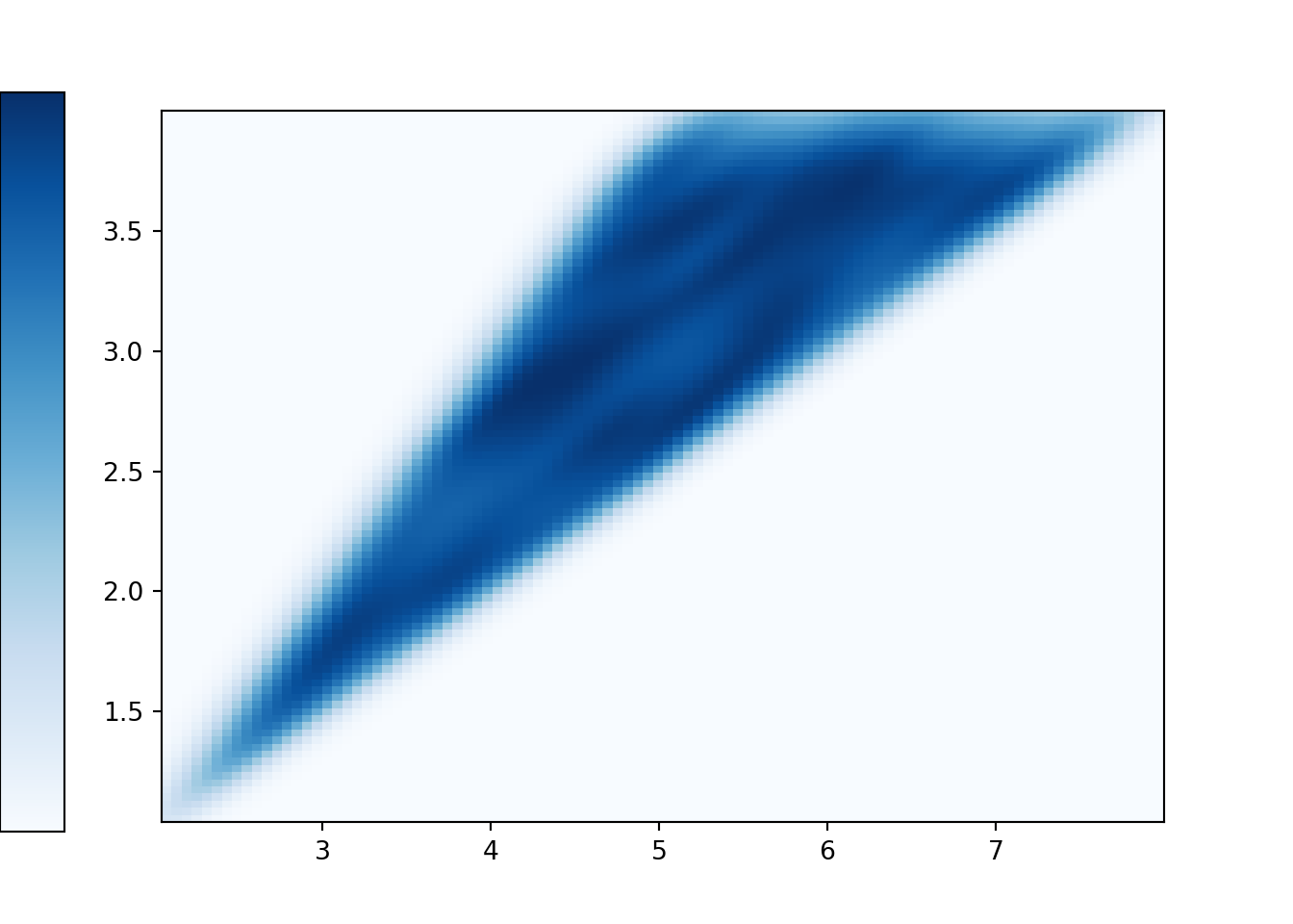
xy.cov()## 0.7417211569275983For two continuous random variables, \(\textrm{E}(XY)\) involves a double integral over possible \((x, y)\) pairs of the product \(xy\) weighted by the joint density. We will see later some strategies for computing \(\textrm{E}(XY)\) and \(\textrm{Cov}(X, Y)\) that avoid double integration.
Example 5.24 What is another name for \(\textrm{Cov}(X, X)\)?
Show/hide solution
The variance of \(X\) is the covariance of \(X\) with itself. \[ \textrm{Cov}(X, X) = \textrm{E}\left((X-\textrm{E}(X))(X-\textrm{E}(X))\right) = \textrm{E}\left((X-\textrm{E}(X))^2\right) = \textrm{Var}(X) \]
5.4.1 Correlation
Example 5.25 The covariance between height in inches and weight in pounds for football players is 96.
- What are the measurement units of the covariance?
- Suppose height were measured in feet instead of inches. Would the shape of the joint distribution change? Would the strength of the association between height and weight change? Would the value of covariance change?
Show/hide solution
- Covariance deals with products, so the covariance is 96 inches\(\times\)pounds.
- A linear rescaling does not change the shape of the distribution or the strength of the association. However, a linear rescaling does relabel the axis and change measurement units. A covariance of 96 inches\(\times\)pounds corresponds to a covariance of 8 feet\(\times\)pounds.
The numerical value of the covariance depends on the measurement units of both variables, so interpreting it can be difficult. Covariance is a measure of joint association between two random variables that has many nice theoretical properties, but the correlation coefficient is often a more practical measure. (We saw a similar idea with variance and standard deviation. Variance has many nice theoretical properties. However, standard deviation is often a better practical measure of variability.)
Definition 5.6 The correlation (coefficient) between random variables \(X\) and \(Y\) is
\[\begin{align*} \textrm{Corr}(X,Y) & = \textrm{Cov}\left(\frac{X-\textrm{E}(X)}{\textrm{SD}(X)},\frac{Y-\textrm{E}(Y)}{\textrm{SD}(Y)}\right)\\ & = \frac{\textrm{Cov}(X, Y)}{\textrm{SD}(X)\textrm{SD}(Y)} \end{align*}\]
The correlation for two random variables is the covariance between the corresponding standardized random variables. Therefore, correlation is a standardized measure of the association between two random variables.
Subtracting the means doesn’t change the scale of the possible pairs of values; it merely shifts the center of the joint distribution. Therefore, correlation is the covariance divided by the product of the standard deviations.
A correlation coefficient has no units and is measured on a universal scale. Regardless of the original measurement units of the random variables \(X\) and \(Y\) \[ -1\le \textrm{Corr}(X,Y)\le 1 \]
- \(\textrm{Corr}(X,Y) = 1\) if and only if \(Y=aX+b\) for some \(a>0\)
- \(\textrm{Corr}(X,Y) = -1\) if and only if \(Y=aX+b\) for some \(a<0\)
Therefore, correlation is a standardized measure of the strength of the linear association between two random variables.
The following plots display a few Bivariate Normal distributions with different correlations.
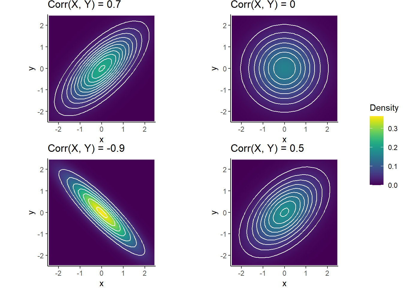
Figure 5.5: Bivariate Normal distributions
Example 5.26 The covariance between height in inches and weight in pounds for football players is 96. Heights have mean 74 and SD 3 inches. Weights have mean 250 pounds and SD 45 pounds. Find the correlation between weight and height.
Show/hide solution
\[ \textrm{Corr}(X, Y) = \frac{\textrm{Cov}(X, Y)}{\textrm{SD}(X)\textrm{SD}(Y)} = \frac{96}{(3)(45)} = 0.71 \]
(The means are useful to have, but they don’t effect the correlation.)
Because correlation is computed between standardized random variables, correlation is not affected by a linear rescaling of either variable. One standard deviation above the mean is one standard deviation above the mean, whether that’s measured in feet or inches or meters.
In many problems we are given the correlation directly and need to find the covariance. Covariance is the correlation times the product of the standard deviations.
\[ \textrm{Cov}(X, Y) = \textrm{Corr}(X, Y)\textrm{SD}(X)\textrm{SD}(Y) \]