8.1 Central limit theorem

Many statistical applications involve random sampling from a population. And one of the most basic operations in statistics is to average the values in a sample. If a sample is selected at random, then the sample mean is a random variable that has a distribution. How does this distribution behave?

Example 8.1 A random sample of $n$ customers at a snack bar is selected, independently. Let $S_n$ by the total dollar amount spent by the $n$ customers in the sample, and let $\bar{X_n}=S_n/n$ represent the sample mean dollar amount spent by the $n$ customers in the sample.

Assume that

40% of customers spend 5 dollars
40% of customers spend 6 dollars
20% of customers spend 7 dollars

Let $X$ denote the amount spent by a single randomly selected customer.

Find $\textrm{E}(X)$. We’ll call this value the population mean $\mu$; explain what this means.
Find $\textrm{SD}(X)$. We’ll call this value the population standard deviation $\sigma$; explain what this means.
Randomly select two customers, independently, and let $X_1$ and $X_2$ denote the amounts spent by the two people selected. Make a table of all possible $(X_1, X_2)$ pairs and their probabilities.
Use the table from the previous part to find the distribution of $\bar{X}_2$. Interpret in words in context what this distribution represents.
Compute and interpret $\textrm{P}(\bar{X}_{2} > 6)$.
Compute $\textrm{E}(\bar{X}_2)$. How does it relate to $\mu$?
There are 3 “means” in the previous part. What do they all mean?
Compute $\textrm{Var}(\bar{X}_2)$ and $\textrm{SD}(\bar{X}_2)$. How do these values relate to the population variance $\sigma^2$ and the population standard deviation $\sigma$?
Describe in words in context what $\textrm{SD}(\bar{X}_2)$ measures variability of.

Solution. to Example 8.1

Show/hide solution

$X$ takes value 5, 6, 7, with probability 0.4, 0.4, 0.2, so $\textrm{E}(X)=5(0.4) + 6(0.4) + 2(0.2)= 5.8$. Over the population of customers, individual customers spend on average 5.8 dollars.
$\textrm{E}(X^2) = 5^2(0.4) + 6^2(0.4) + 2^2(0.2)= 34.2$ so $\textrm{Var}(X) = E(X^2) - (E(X))^2 = 0.56$ squared-dollars and $\textrm{SD}(X) = \sqrt{0.56} = 0.748$ dollars. Over the population of customers, amounts spent by individual customers deviate from the mean on average by about 0.75 dollars.

See the table below. Since $X_1$ and $X_2$ are independent, the probability of any pair is the product of the marginal probabilities.

$X_1$	$X_2$	Probability	$\bar{X}_2$
5	5	(0.4)(0.4)=0.16	5.0
5	6	(0.4)(0.4)=0.16	5.5
5	7	(0.4)(0.2)=0.08	6.0
6	5	(0.4)(0.4)=0.16	5.5
6	6	(0.4)(0.4)=0.16	6.0
6	7	(0.4)(0.2)=0.08	6.5
7	5	(0.2)(0.4)=0.08	6.0
7	6	(0.2)(0.4)=0.08	6.5
7	7	(0.2)(0.2)=0.04	7.0

Just collapse the table from the previous part. This is the distribution of sample mean amount spent over many samples of 2 customers.

$\bar{x}_2$ $\textrm{P}(\bar{X}_2 = \bar{x}_2)$

5.0 0.16

5.5 0.32

6.0 0.32

6.5 0.16

7.0 0.04
$\textrm{P}(\bar{X}_{2} > 6) = 20$. In 20% of samples of size 2 the sample mean income is greater than 6 dollars.
$\textrm{E}(\bar{X}_2)=5(0.16) + 5.5(0.32) + 6(0.32) + 6.5(0.16) + 7(0.04) = 5.8$. We see that $\textrm{E}(\bar{X}_2)=\mu$.
Over many samples of size 2, the average of the sample means is equal to the population mean.
$\textrm{E}(\bar{X}_2^2)=5^2(0.16) + 5.5^2(0.32) + 6^2(0.32) + 6.5^2(0.16) + 7^2(0.04) = 33.92$ and $\textrm{Var}(\bar{X}_2) = \textrm{E}(\bar{X}_2^2) - (\textrm{E}(\bar{X}_2))^2 = 33.92 - 5.8^2 = 0.28 = 0.56 / 2$, and $\textrm{SD}(\bar{X}_2) = \sqrt{0.28} = 0.529 = \sqrt{0.748} / \sqrt{2}$. \[\begin{align*} \textrm{Var}(\bar{X}_2) & = \frac{\textrm{Var}(X)}{2}\\ \textrm{SD}(\bar{X}_2) & = \frac{\textrm{SD}(X)}{\sqrt{2}}\\ \end{align*}\] 1.$\textrm{SD}(\bar{X}_2)$ measures the sample-to-sample variability of sample mean amount spent over many samples of size 2 customers. Over many samples of 2 customers, the sample mean amount spent deviates from the population mean amount spent by about 0.53 dollars on average.

\(\bar{x}_2\)	\(\textrm{P}(\bar{X}_2 = \bar{x}_2)\)
5.0	0.16
5.5	0.32
6.0	0.32
6.5	0.16
7.0	0.04

Many problems in statistics involve sampling from a population. The population distribution describes the distribution of values of a variable over all individuals in the population. The population mean, denoted $\mu$, is the average of the values of the variable over all individuals in the population.
The population standard deviation, denoted $\sigma$, is the standard deviation of all the individual values in the population.

A (simple) random sample of size $n$ is a collection of random variables $X_1,\ldots,X_n$ that are independent and identically distributed (i.i.d.)

Independence assumes individuals are selected for the sample independently of one another (think of sampling with replacement, or sampling without replacement from a very large population)
Identically distributed assumes all individuals are selected from the same population, so all the individual values are selected from the same population distribution.

The sample mean is \[ \bar{X}_n = \frac{X_1 + \cdots + X_n}{n} = \frac{S_n}{n}, \] where $S_n=X_1+\cdots+X_n$ is the sum (total) of values in the sample. Because the sample is randomly selected, the sample mean $\bar{X}_n$ is a random variable that has a distribution. This distribution describes how sample means vary from sample-to-sample over many random samples of size $n$.

Over many random samples, sample means do not systematically overestimate or underestimate the population mean. (We say that the sample mean $\bar{X}$ is an unbiased estimator of the population mean $\mu$.) \[ \textrm{E}(\bar{X}_n) = \mu \]

Variability of sample means depends on the variability of individual values of the variable; the more the values of the variable vary from individual-to-individual in the population, the more the sample means will vary from sample-to-sample. However, sample means are less variable than individual values of the variable. Furthermore, the sample-to-sample variability of sample means decreases as the sample size increases \[\begin{align*} \textrm{Var}(\bar{X}_n) & = \frac{\sigma^2}{n}\\ \textrm{SD}(\bar{X}_n) & = \frac{\sigma}{\sqrt{n}} \end{align*}\] Over many random samples, sample means from larger random samples vary less, from sample to sample, than sample means from smaller random samples. The standard deviation of sample means decreases as the sample size increases, but this reduction in SD follows a “square root rule”. For example, if the sample size is increased by a factor of 4, then the sample-to-sample standard deviation of the sample mean is reduced by a factor of $\sqrt{4} = 2$.

Given the population mean $\mu$ and population standard deviation $\sigma$, the above formulas provide the mean and standard deviation of the sample-to-sample distribution of sample means for any sample size. But what about the shape of the sample-to-sample distribution of sample means?

In Example 8.1 we found the distribution of sample means by enumerating all possible samples, but this strategy is unfeasible in almost all problems. Therefore, we need other ways of finding or approximating the distribution of $\bar{X}_n$. As always, simulation is an excellent way to approximate distributions.

Before simulating sample means, we first simulate individual values. The following simulates the population distribution of individual values of the variable $X$ in Example 8.1.

population = BoxModel([5, 6, 7], probs = [0.4, 0.4, 0.2])

X = RV(population)

x = X.sim(10000)

x

Index	Result
0	5
1	5
2	6
3	5
4	6
5	7
6	6
7	7
8	5
...	...
9999	5

x.mean(), x.var(), x.sd()

## (5.7867, 0.55120311, 0.7424305422058012)

x.plot()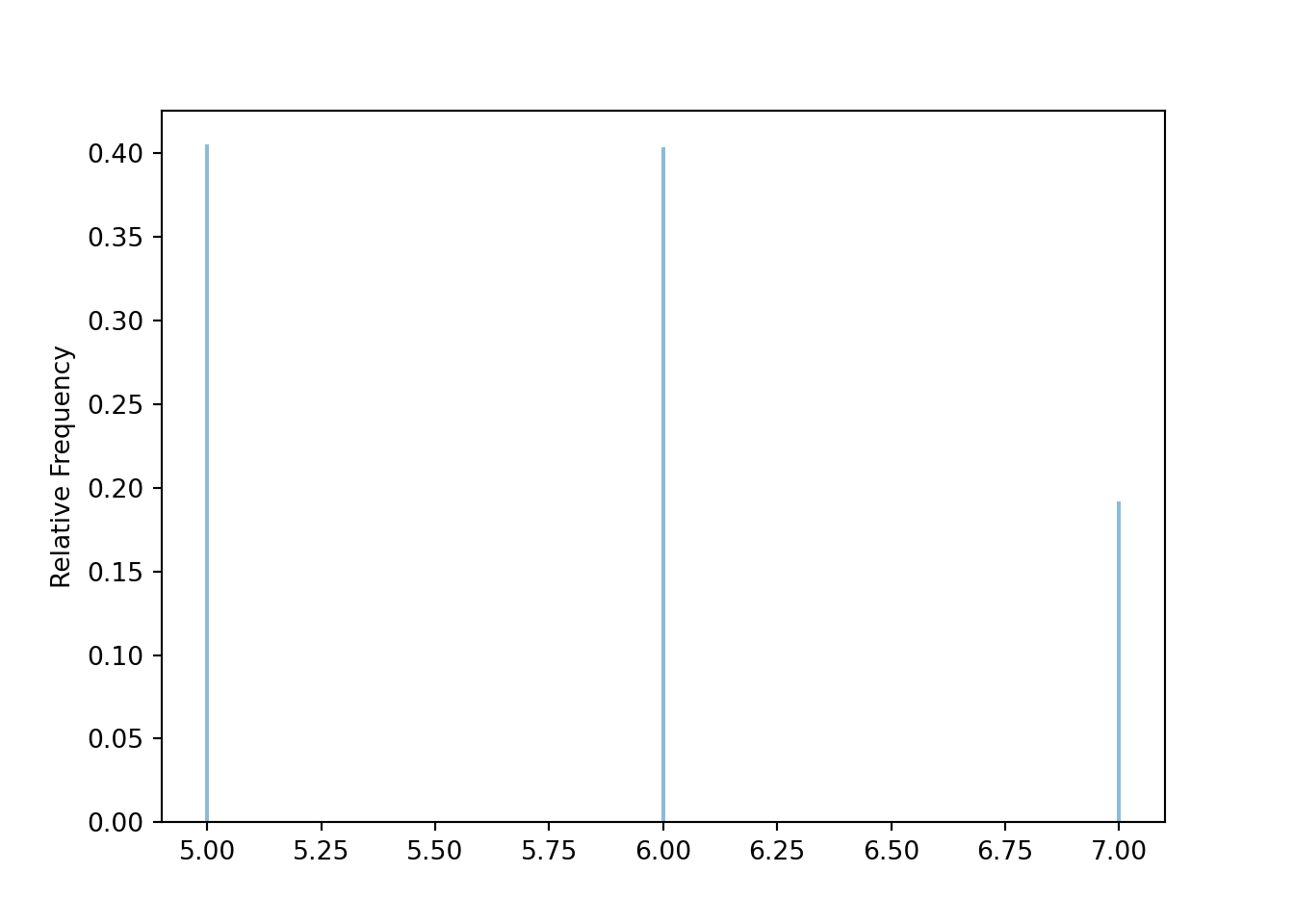

Now we simulate sample means for many samples of size 2. The random variable Xbar below takes n independent simulated values from the population (population ** n) and returns the sample mean. The sim(10000) command simulates 10000 samples of size n and computes the sample mean for each of these 10000 samples.

population = BoxModel([5, 6, 7], probs = [0.4, 0.4, 0.2])

n = 2

Xbar = RV(population ** n, mean)

xbar = Xbar.sim(10000)

xbar

Index	Result
0	7.0
1	6.0
2	6.0
3	5.0
4	6.0
5	5.5
6	5.5
7	6.0
8	5.5
...	...
9999	6.0

xbar.mean(), xbar.var(), xbar.sd(), xbar.count_gt(6) / xbar.count()

## (5.8029, 0.27955159, 0.5287263848154355, 0.202)

xbar.plot()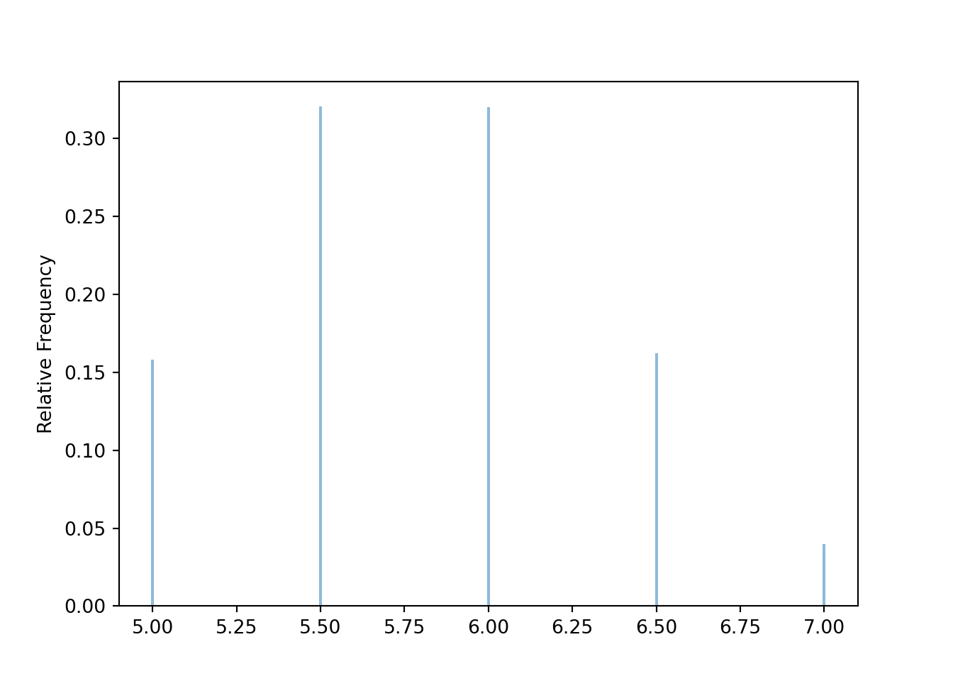

The simulation results are consistent with our work in Example 8.1.

In general, the exact shape of the distribution of $\bar{X}_n$ depends on the shape of the population distribution of individual values, in a complicated way¹⁴³. Fortunately, the approximate shape of the distribution of $\bar{X}_n$ often follows a specific distribution that we’re well acquainted with.

Example 8.2 Continuing Example 8.1. Now suppose we take a random sample of 30 customers; consider $n=30$ and $\bar{X}_{30}$.

Find $\textrm{E}(\bar{X}_{30})$, $\textrm{Var}(\bar{X}_{30})$, and $\textrm{SD}(\bar{X}_{30})$.
What does $\textrm{SD}(\bar{X}_{30})$ measure the variability of?
Use simulation to determine the approximate shape of the distribution of $\bar{X}_{30}$.
Simulation shows that $\bar{X}_{30}$ has an approximate Normal distribution. Use this Normal distribution to approximate $\textrm{P}(\bar{X}_{30} > 6)$, and interpret the probability.

Solution. to Example 8.2

Show/hide solution

It’s the same population as before so the population mean is $\mu = 5.8$ and the population standard deviation is $\sigma = \sqrt{0.56} = 0.748$. Therefore, $\textrm{E}(\bar{X}_{30}) = \mu = 5.8$, $\textrm{Var}(\bar{X}_{30}) = \sigma^2/n = 0.56/30 = 0.019$, and $\textrm{SD}(\bar{X}_{30})=\sigma/\sqrt{30} = 0.137$.
$\textrm{SD}(\bar{X}_{30})= 0.137$ measures the sample-to-sample variability of sample means over many samples of size 30. Sample means deviate from the population mean by about 0.137 (dollars) on average. Notice that the sample-to-sample variability of sample means is smaller for samples of size 30 than for samples of size 2.
See simulation results below. The distribution of $\bar{X}_{30}$ is approximately Normal with a mean of 5.8 and a standard deviation of 0.137. This distribution describes the sample-to-sample pattern of variability of sample means over many samples of size 30.
The value 6 is $(6-5.8)/0.137=1.46$ standard deviations above the mean of the Normal distribution, so $\textrm{P}(\bar{X}_{30} > 6)$ is about 0.07. In about 7% of samples of size 30 the sample mean amount spent per customer is greater than 6 dollars.

Now we revise our simulation to simulate samples of size 30 and their sample means.

population = BoxModel([5, 6, 7], probs = [0.4, 0.4, 0.2])

n = 30

Xbar = RV(population ** n, mean)

xbar = Xbar.sim(10000)

xbar

Index	Result
0	5.933333333333334
1	6.0
2	5.833333333333333
3	5.7
4	5.833333333333333
5	5.866666666666666
6	5.833333333333333
7	5.866666666666666
8	5.8
...	...
9999	5.766666666666667

Compare the simulation based approximations of $\textrm{E}(\bar{X}_{30})$, $\textrm{Var}(\bar{X}_{30})$, and $\textrm{SD}(\bar{X}_{30})$ to the their theoretical values determined above.

xbar.mean(), xbar.var(), xbar.sd()

## (5.800353333333334, 0.01888409737777777, 0.13741942139951605)

Our simulation shows that the sample-to-sample distribution of sample means over many samples of size 30 has an approximate Normal shape.

xbar.plot()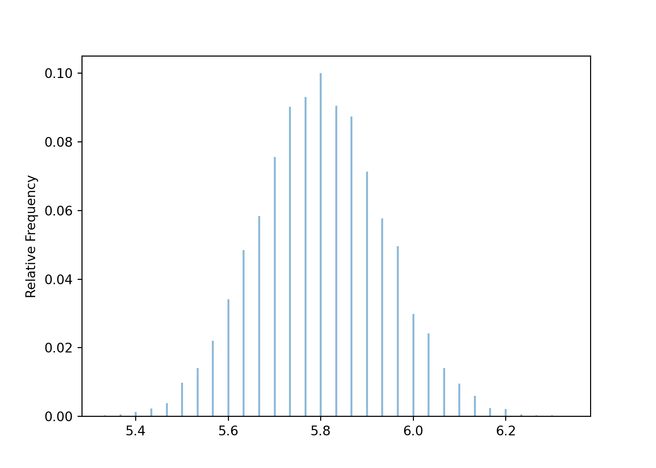

Compare the simulation based approximation of $\textrm{P}(\bar{X}_{30} > 6)$ with the Normal approximation¹⁴⁴.

xbar.count_gt(6) / xbar.count(), 1 - Normal(5.8, sqrt(0.56) / sqrt(n)).cdf(6)

## (0.06, 0.07161745376233464)

The previous example illustrates that if the sample size is large enough then the sample-to-sample distribution of sample means will be approximately Normal even if the population distribution of individual values is not. This idea is formalized in the Central Limit Theorem.

The (Standard) Central Limit Theorem¹⁴⁵. Let $X_1,X_2,\ldots$ be independent and identically distributed (i.i.d.) random variables with finite mean $\mu$ and finite standard deviation¹⁴⁶ $\sigma$. Then¹⁴⁷ $\bar{X}_{n}$ has an approximate Normal distribution, if $n$ is large enough. That is, \[ \text{$\bar{X}_n$ has an approximate $N\left(\mu,\frac{\sigma}{\sqrt{n}}\right)$ distribution, if $n$ is large enough.} \]

We can switch back and forth between sums and averages: the sum is just the sample mean times the sample size, $S_n = n\bar{X}_n$. Multiplying $\bar{X}_n$ by the number $n$ will not change the general shape of the distribution, just its mean and standard deviation. So the CLT also says that the sum $S_{n}$ has an approximate Normal distribution, if $n$ is large enough. That is, \[ \text{$S_n$ has an approximate $N(n\mu,\sigma\sqrt{n})$ distribution, if $n$ is large enough} \]

The CLT says that if the sample size is large enough, the sample-to-sample distribution of sample means (or sums) is approximately Normal, regardless of the shape of the population distribution. A natural question: “How large is large enough?” The short answer: it depends. We’ll elaborate after the following example.

Example 8.3 Continuing Example 8.1. Now suppose that each customer spends 5 dollars with probability 0.4, 6 with probability 0.4, 7 with probability 0.19, and 30 with probability 0.01 (maybe they treat a few friends).

Use simulation to approximate the distribution of $\bar{X}_{30}$; is it approximately Normal?
Use simulation to approximate the distribution of $\bar{X}_{100}$; is it approximately Normal?
Use simulation to approximate the distribution of $\bar{X}_{300}$; is it approximately Normal?

Solution. to Example 8.3

Show/hide solution

Note that for this population $\mu = 6.03$ and $\sigma=2.52$

See the simulation results below. The distribution doesn’t look anything like a Normal distribution when $n=30$.

When $n=100$ the distribution is closer to Normal than when $n=30$, but still definitely not Normal. The individuals who spend 30 dollars throw off the averages, even when the sample size isn’t super small.

When the sample size is large, the outliers have less affect on the mean and the overall average characteristics take over. For samples of size 300 the distribution of sample means looks much closer to Normal, but some asymmetry is still present.

The following simulation uses the population distribution from Example 8.3. The distribution of sample means is not Normal when $n=30$. (The distinct “humps” basically correspond to samples with no people who spent 30 dollars, samples with exactly 1 person who spent 30 dollars, samples with exactly 2 people who spent 30 dollars, etc)

population = BoxModel([5, 6, 7, 30], probs = [0.4, 0.4, 0.19, 0.01])

n = 30

Xbar = RV(population ** n, mean)

xbar = Xbar.sim(10000)

xbar

Index	Result
0	5.533333333333333
1	5.933333333333334
2	5.533333333333333
3	6.733333333333333
4	6.6
5	7.666666666666667
6	5.8
7	5.9
8	5.9
...	...
9999	7.533333333333333

xbar.plot()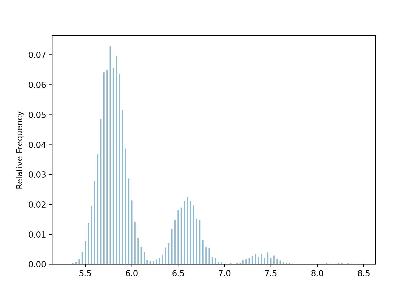

For samples of size 100, the distribution is sample means is less distinctly “humpy”, but still far from Normal.

population = BoxModel([5, 6, 7, 30], probs = [0.4, 0.4, 0.19, 0.01])

n = 100

Xbar = RV(population ** n, mean)

xbar = Xbar.sim(10000)

xbar.plot()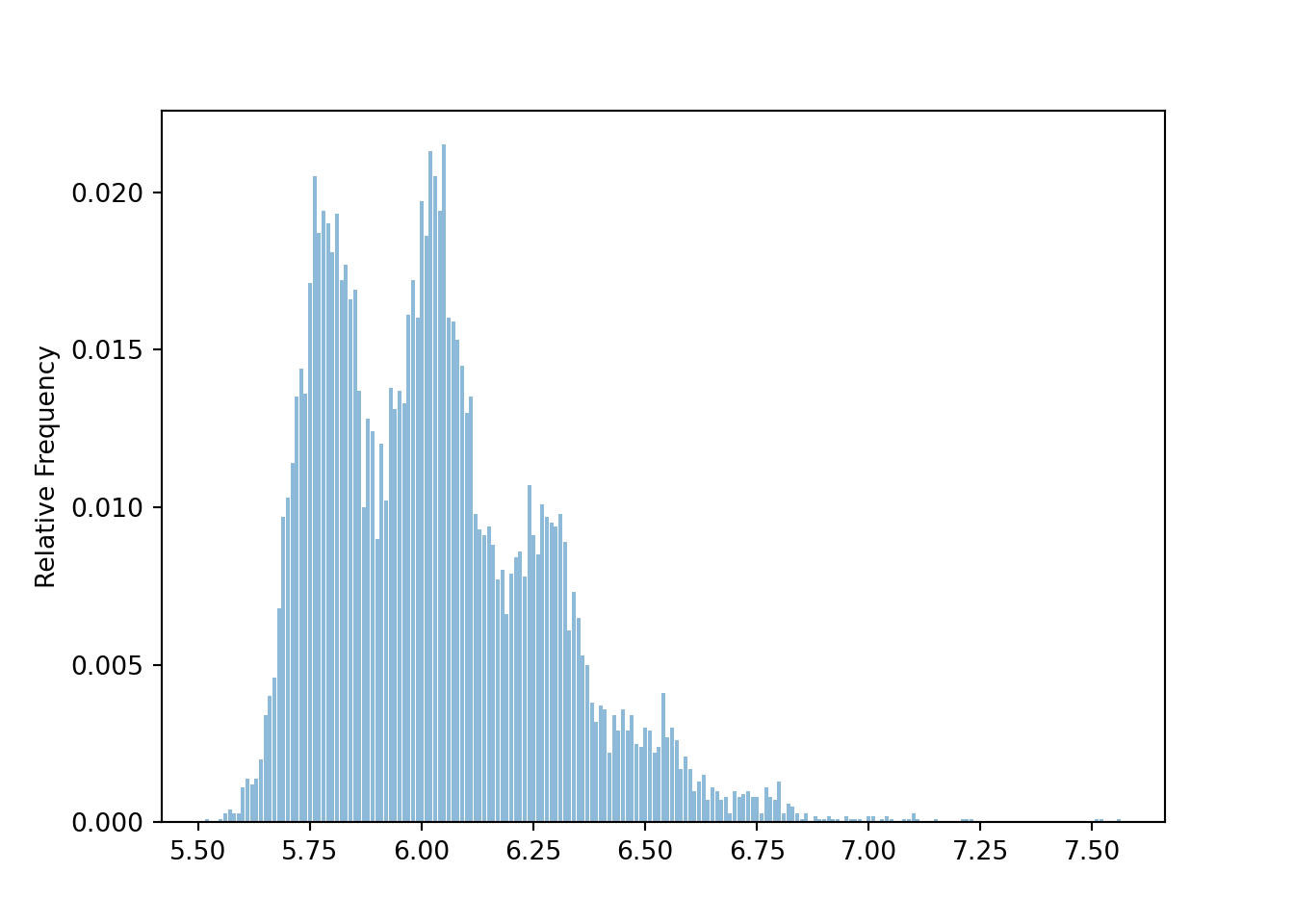

For samples of size 300, the humps have disappeared, but the distribution of sample means is still a little right skewed compared with a Normal distribution.

population = BoxModel([5, 6, 7, 30], probs = [0.4, 0.4, 0.19, 0.01])

n = 300

Xbar = RV(population ** n, mean)

xbar = Xbar.sim(10000)

xbar.plot('hist')
Normal(6.03, 2.52 / sqrt(n)).plot()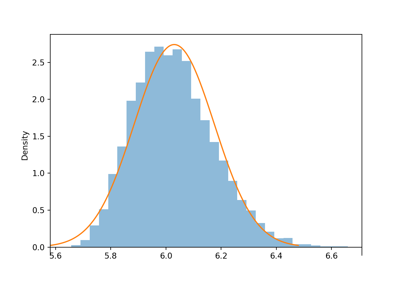

The previous example is an early cautionary tale. There is no magic number¹⁴⁸ for how large the sample size needs to be for the CLT to kick in.

The CLT says that if the sample size is large enough, the sample-to-sample distribution of sample means is approximately Normal, regardless of the shape of the population distribution. However, the shape of the population distribution — which describes the distribution of individual values of the variable — does matter in determining how large is large enough.

If the population distribution is Normal, then the sample-to-sample distribution of sample means is Normal for any sample size.
If the population distribution is “close to Normal” — e.g., symmetric, light tails, single peak — then smaller samples sizes are sufficient for the sample-to-sample distribution of sample means to be approximately Normal.
If the population distribution is “far from Normal” — e.g., severe skewness, heavy tails, extreme outliers, multiple peaks — then larger sample sizes are required for the sample-to-sample distribution of sample means to be approximately Normal.

You should certainly be aware that some population distributions require a large sample size for the CLT to kick in. However, in many situations the sample-to-sample distributions of sample means is approximately Normal even for small or moderate sample sizes.

Clicking on the following will take you to a Colab notebook that conducts a simulation of samples means like the ones earlier in the section. You can experiment with different population distributions and sample sizes to see the Central Limit Theorem in action.

The Central Limit Theorem provides a relatively simple and easy way to approximate probabilities in a wide variety of problems that involve sums or averages of many independent random quantities. In some of the next few examples we’ll work with sample means $\bar{X}_n$; in the others, sums $S_n$. Either way is fine; you just need to make sure you use the appropriate mean ($\mu$ versus $n\mu$) and standard deviation ($\sigma/\sqrt{n}$ versus $\sigma/\sqrt{n}$) for the Normal distribution. To avoid confusion, you might want to translate every problem in terms of $\bar{X}_n$.

Example 8.4 The number of free throws that a particular basketball player attempts in a game has a Poisson distribution with parameter 2.7. Approximate the probability that the player attempts more than 60 free throws in the next 20 games.

Solution. to Example 8.4

Show/hide solution

Each $X_i$ represents the number of free throws in a single game. The population distribution is the Poisson(2.7) distribution, since this describes the distribution of the number of free throw attempts in individual games. The mean of the Poisson(2.7) distribution is 2.7, so the population mean is $\mu = 2.7$. The standard deviation of the Poisson(2.7) distribution is $\sqrt{2.7} = 1.64$, so the population standard deviation is $\sigma = 1.64$.

The total number of free throw attempts in the next 20 games is $S_{20}$. Assuming $n=20$ is large enough for the CLT to kick in for a Poisson(2.7) population distribution, $S_{20}$ has an approximate Normal distribution with mean $n\mu = 20(2.7) = 54$ and standard deviation $\sigma\sqrt{n} = 1.64\sqrt{20} = 7.35$.

We want $\textrm{P}(S_{20} > 60)$. A value of 60 is $(60-54)/7.35 = 0.82$ standard deviations above the mean. Using a Normal distribution approximation, the probability is approximately 0.21. The player is about 4 times more likely than not to attempt at most 60 free throws in the next 20 games.

Is a sample size of 20 large enough for a Normal approximation in the previous problem? Here is our population distribution, the Poisson(2.7) distribution.

Poisson(2.7).plot()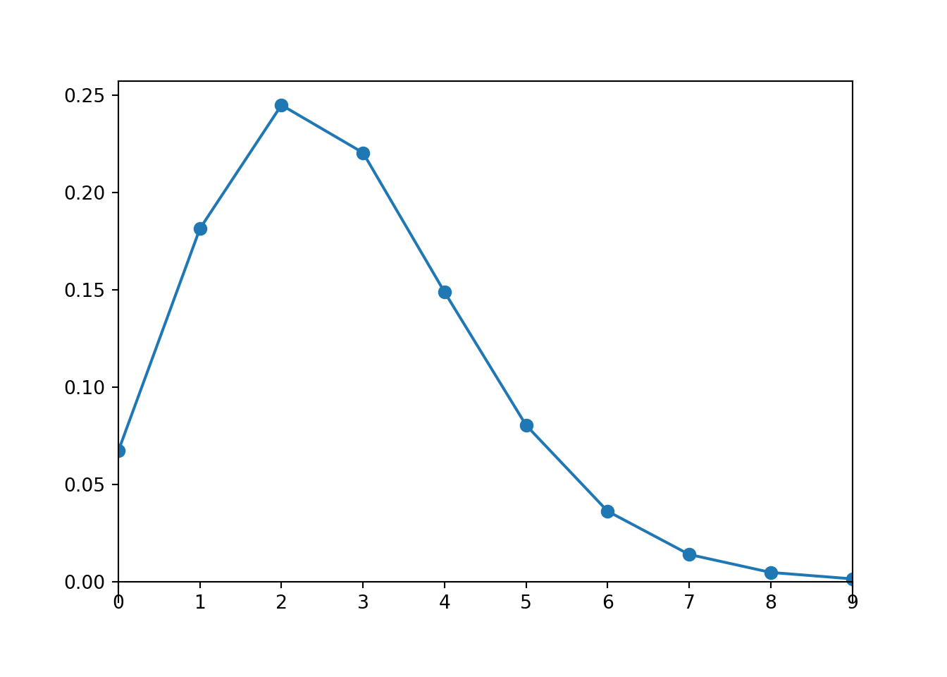

A Poisson(2.7) distribution is not very skewed, does not produce many extreme values, and has a single peak, so maybe a small sample size like 20 is ok for the distribution of sample means to be approximately Normal. Simulation confirms this.

population = Poisson(2.7)

n = 20

S = RV(population ** n, sum)

s = S.sim(10000)

s.count_gt(60) / s.count()

## 0.1873

s.plot('hist')
Normal(2.7 * n, sqrt(2.7) * sqrt(n)).plot()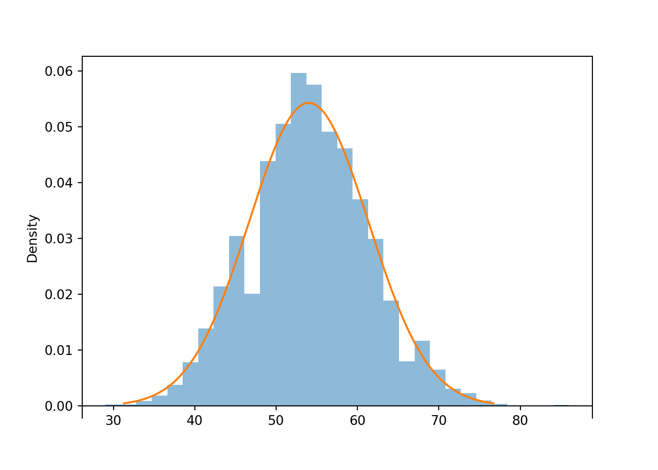

In the previous problem we could have just used Poisson aggregation: $S_{20}$ has a Poisson(54) distribution. The probability from the Normal approximation is reasonably close¹⁴⁹ to the theoretical probability that Poisson(54) distribution yields a value greater than 60. Of course, the simulated relative frequency of sums greater than 60 is also close to the theoretical probability.


1 - Poisson(2.7 * 20).cdf(60)

## 0.18675483040641572

Example 8.5 Ten independent resistors are connected in series. Each has a resistance Uniformly distributed between 215 and 225 ohms, independently. Compute the probability that the mean resistance of this series system is between 219 and 221 ohms.

Solution. to Example 8.5

Show/hide solution

Each $X_i$ represents the resistance of a single resistor The population distribution is the Uniform(215, 225) distribution, since this describes the distribution of resistances for individual resistors. The mean of the Uniform(215, 225) distribution is 220, so the population mean is $\mu = 220$ ohms. The standard deviation of the Uniform(215, 225) distribution is $(225-215)/\sqrt{12} = 2.89$, so the population standard deviation is $\sigma = 2.89$ ohms.

The mean resistance of the 10 resistors is $\bar{X}_{10}$. Assuming $n=10$ is large enough for the CLT to kick in for a Uniform(215, 225) population distribution, $\bar{X}_{10}$ has an approximate Normal distribution with mean $\mu = 220$ and standard deviation $\sigma/\sqrt{n} = 2.89/\sqrt{10} = 0.91$.

We want $\textrm{P}(219 < \bar{X}_{10} < 221)$. That is, we want the probability that $\bar{X}_{10}$ is within $(221 - 220) / 0.91 = 1.09$ standard deviations of the mean. Using a Normal distribution approximation, the probability is approximately 0.73.

Is a sample size of 10 large enough for a Normal approximation in the previous problem? The Uniform(215, 225) distribution certainly isn’t Normal, but it is symmetric, and it is bounded so it never produces super extreme values. Simulation suggests that for a Uniform population, even a sample size of 10 is large enough for the sample-to-sample distribution of sample means to be approximately Normal.

population = Uniform(215, 225)

n = 10

Xbar = RV(population ** n, mean)

xbar = Xbar.sim(10000)

abs(xbar - 220).count_lt(1) / xbar.count()

## 0.7216

xbar.plot('hist')
Normal(220, (10 / sqrt(12)) / sqrt(n)).plot()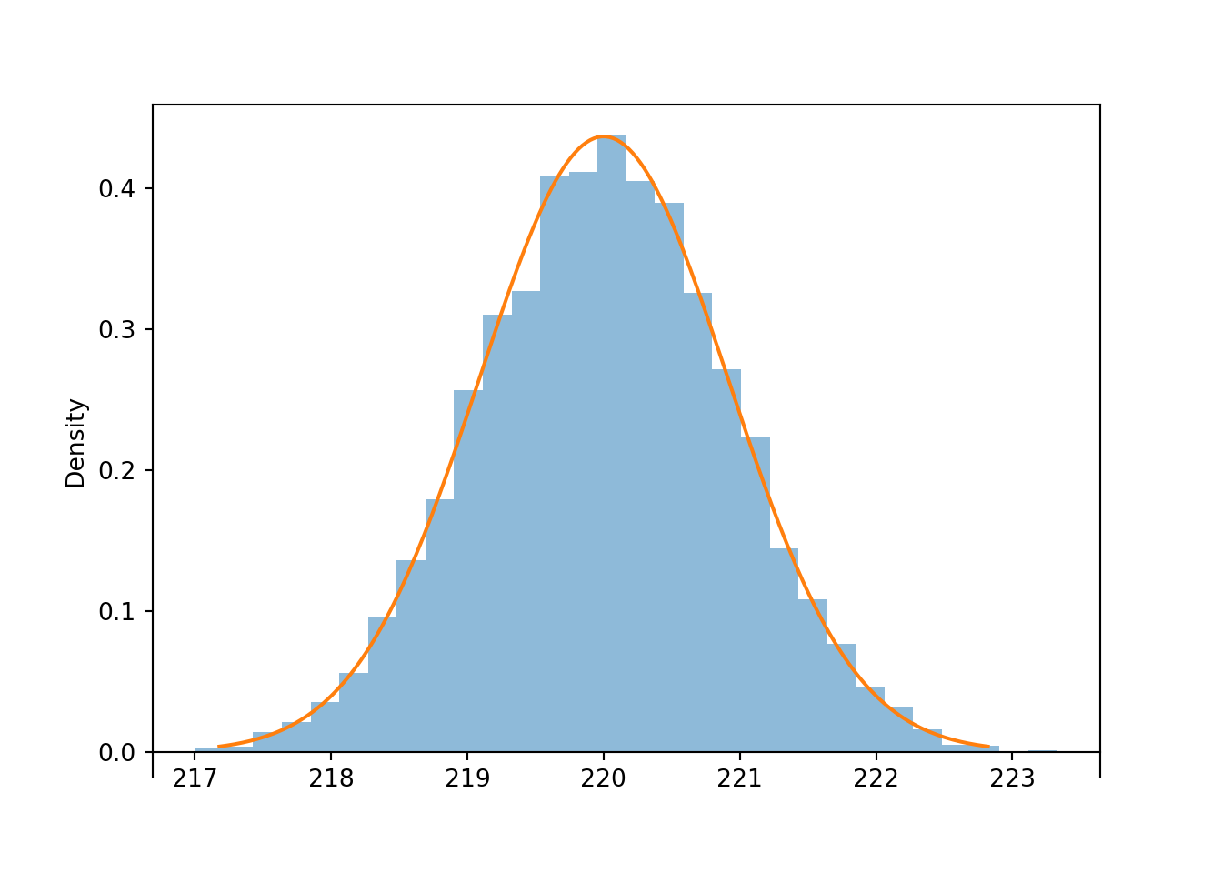

Example 8.6 A fair six-sided die is rolled until the total sum of all rolls exceeds 300. Approximate the probability that at least 80 rolls are necessary.

Solution. to Example 8.6

Show/hide solution

To apply the CLT we need a fixed sample size. However, in this problem the sample size is random, so it’s not immediately clear how to apply the CLT. The key is to represent the event of interest involving the random number of rolls as an equivalent event involving a fixed number of rolls. Logically, at least 80 rolls are necessary for the sum to exceed 300 if and only if the sum of the first 79 rolls is at most 300. So we want $\textrm{P}(S_{79} \le 300)$, where $S_{79}$ is the sum of the first 79 rolls.

Each $X_i$ represents a single roll. The population distribution is the DiscreteUniform(1, 6) distribution, that is, the distribution where the values $1, \ldots, 6$ are equally likely. The population mean is $\mu = 1(1/6) + \cdots + 6(1/6) = 3.5$ and the population standard deviation is $\sigma = \sqrt{(1^2(1/6) + \cdots + 6^2(1/6)) - 3.5^2}=\sqrt{35/12} = 1.708$.

The sum of the first 79 rolls is $S_{79}$. Assuming $n=79$ is large enough for the CLT to kick for this population distribution, $S_{79}$ has an approximate Normal distribution with mean $n\mu = 79(3.5) = 276.5$ and standard deviation $\sigma\sqrt{n} = 1.708\sqrt{79} = 15.18$.

We want $\textrm{P}(S_{79} \le 300)$. The value 300 is $(300-276.5)/15.18 = 1.55$ standard deviations above the mean. Using a Normal distribution approximation, the probability is approximately 0.94.

In the previous problem, we applied the CLT to the sum of the first 79 rolls. Simulation confirms that the distribution of $S_{79}$ is approximately Normal.

population = BoxModel([1, 2, 3, 4, 5, 6])

n = 79

S = RV(population ** n, sum)

s = S.sim(10000)

s.count_leq(300) / s.count()

## 0.9468

s.plot('hist')
Normal(3.5 * n, 1.708 * sqrt(n)).plot()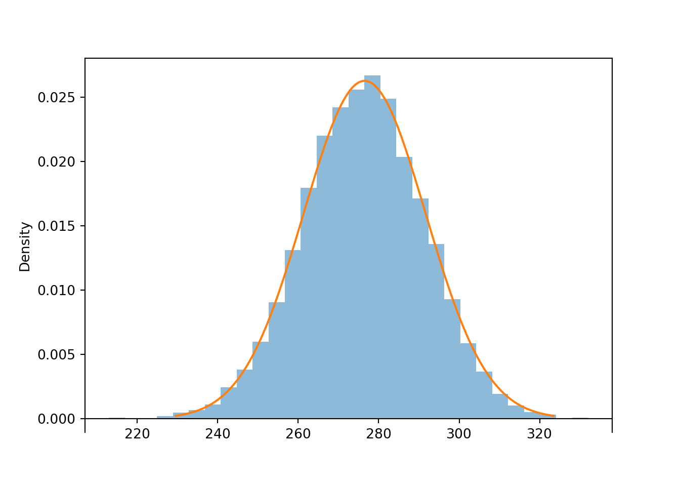

Below we simulate the distribution of the random number of rolls needed for the sum to exceed 300.

t = 300

def sum_until_t(omega):
    trials_so_far = []
    for i, w in enumerate(omega):
        trials_so_far.append(w)
        if sum(trials_so_far) > t:
            return i + 1 
        
P = BoxModel([1, 2, 3, 4, 5, 6], size=inf)
X = RV(P, sum_until_t)
x = X.sim(10000)

plt.figure()
x.plot()
plt.show()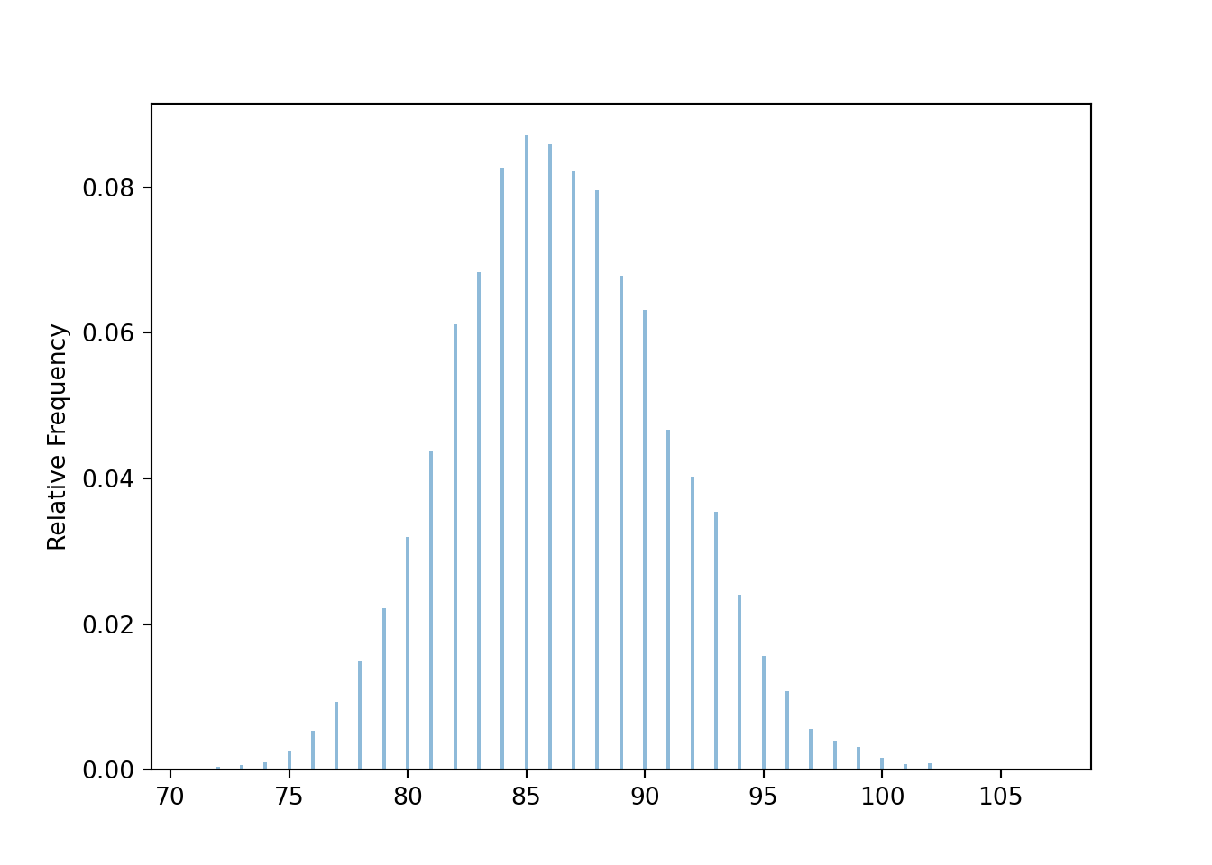

x.mean(), x.sd(), x.count_geq(80) / x.count()

## (86.489, 4.585333030435194, 0.9433)

Example 8.7 Suppose that average annual income for U.S. households is about $100,000, and that the standard deviation of income is about $230,000.

What can you say about the probability that a single randomly selected household has an income above $120,000?
Donny Don’t says: “Since a sample size of one million is extremely large, the CLT says that the incomes in a sample of one million households should follow a Normal distribution”. Do you agree? If not, explain to Donny what the CLT does say.
Use the CLT to approximate the probability that in a sample of 1000 households the sample mean income is above $120,000.
Donny says: “Wait, the distribution of household income is highly skewed to the right. Wouldn’t it be more appropriate to use the sample median than the sample mean”? Do you agree? Explain.

Solution. to Example 8.7

Show/hide solution

Not much¹⁵⁰. The mean and the standard deviation don’t tell us much¹⁵¹ about the shape of the distribution. We know from experience that distributions of incomes are highly skewed to the right, but we don’t know what percentile an income of $120,000 represents, and there is no way to figure out it based on the mean and standard deviation alone.
Donny is misinterpreting the CLT. The CLT doesn’t say anything about the shape of the population distribution of individual household incomes. We know from experience that the population distribution of incomes will be fairly skewed to the right. A random sample of one million households should be reasonably representative of the population, so we would expected the distribution of incomes in the sample to have a shape similar to the population distribution of incomes; we would expect the distribution of the individual incomes in the sample to be skewed to the right. The CLT says that if we were to take many random samples of one million households each and compute the mean income for each sample, then the sample-to-sample distribution of sample means would be approximately Normal.
Assuming that a sample size of 1000 is large enough for the CLT to kick in, the sample-to-sample distribution of sample mean income over many samples of 1000 households will be approximately Normal with mean 100,000 and standard deviation $230000/\sqrt{1000} = 7273$. The value 120,000 is $(120000-100000)/7273 = 2.75$ standard deviations above the mean. So the probability is about 0.003. If population mean income is $100,000 then we would see a sample mean income greater than $120,000 in only 0.3% of samples of 1000 households.
Donny has a good point! Means are commonly used as a measure of “center” of a distribution. The CLT makes sample means relatively easy to work with. But just because sample means are easy to analyze, doesn’t make them the right thing to analyze. For incomes, it is often more appropriate to represent center with a median. For example, in 2019 the mean annual household income in the U.S. was about $100,000 but the median was about $70,000; that’s a big difference! In particular, as a single number, $70,000 is much more representative of a “typical” annual household income than $100,000.

Be careful to distinguish between what the CLT does say, and what it doesn’t say. The CLT doesn’t say anything about the shape of the population distribution of individual values of the variable; it can be anything. Randomly selected samples tend to be representative of the population they’re sampled from, so we expect the shape of the distribution of individual values in the sample to resemble the shape of the distribution of individual values in the population, regardless of the sample size. Over many samples, the distribution of individual values within each sample will resemble the population distribution. For example, if the population distribution has an Exponential shape, then the distribution of values in any single randomly selected sample will tend to have a roughly Exponential shape.

The CLT applies to how sample means behave over many samples, not what happens within any single sample. If $n$ is large enough, then over many samples of size $n$ the sample-to-sample distribution of sample means will be approximately Normal, regardless of the shape of the population distribution of individual values of the variable.

You might say: “Why do we need the CLT? We can always approximate the distribution of sample means with a simulation”. (And a simulation often provides a better approximation than a Normal approximation, as illustrated by Example 8.4.) True! And we certainly want to encourage you to use simulation as much as possible! But the CLT is definitely something well worth knowing; here are just a few reasons.

The CLT is amazing. The sample-to-sample distribution of sample means is approximately Normal regardless of the shape of the population distribution.
Really, the CLT is amazing. The simple process of averaging (or adding) “normalizes” random quantities. If you take a bunch of random quantities and average them, the distribution of the average will be roughly Normal.
The CLT provides some justification for the ubiquity of Normal distributions. Many quantities in the natural world follow a Normal distribution. We can often think of these measurements as a sum of smaller quantities, and so the CLT provides some justification for why the measurements follow a Normal distribution.
The CLT is the backbone of many statistical methods, including many widely used confidence interval and hypothesis testing procedures.
The CLT is historically important. The CLT was indispensable in the times before modern computing.
Even when we can approximate via simulation, the CLT provides relatively simple and easy ballpark estimates in a wide variety of problems.

Why should the CLT be true? We have seen examples providing evidence that the CLT is true, but it is far from obvious just why the CLT is true. Unfortunately, there is not an easy intuitive explanation, but we’ll try our best to provide an idea of why the CLT is true.

The CLT says something about the distribution of an average (or sum) of a large number of terms. Here we’ll focus on averages; sums can be treated similarly. Understanding why the theorem should be true involves the following key ideas in sequence. Try to convince yourself of the following (“if 1 is true then 2 has to be true”, “if 2 is true then 3 has to be true”, etc).

If there are enough independent random quantities being averaged then the contribution to the overall average of any one particular quantity is small.
Since the contribution of each individual value to the overall average is small, the particular form of the population distribution — which describes how individual values behave — is not that important. What matters is what happens on average.
If $n$ is large enough then only the mean and standard deviation of the population distribution matter in terms of the distribution of the average. The population mean identifies “typical” values of the sample mean; the population SD identifies the size of the “typical deviation” from the typical value. These two numbers are enough to characterize what happens “on average”. Therefore, two different population distributions with the same mean and standard deviation will give rise to the same distribution of the sample mean if the sample size is large enough.
The distribution of the averages in standardized units is the same for every population if $n$ is large enough. So there is just one possible distribution for the averages in standard units, if $n$ is large enough.
We only need to find the distribution of the average in standard units for one population distribution to find the approximate distribution if $n$ is large for all population distributions. Consider a Normal population distribution. Unrelated to the CLT, we know that if the population distribution is Normal exactly then the distribution of the average is Normal exactly, for any sample size.

Putting it all together gives the conclusion of the CLT.

Before elaborating on these steps, consider an analogy. Suppose you have the following sum, \[ 10 + 1 + 1 + 1 + 1 + 1 + \cdots \] where you just keep adding 1’s forever. Now look at the average of the first $n$ terms: \[ \frac{10 + 1 + 1 + 1 + \cdots +1}{n} = \frac{10}{n} + \frac{1}{n}+ \frac{1}{n}+ \frac{1}{n}+ \cdots + \frac{1}{n}. \] If $n$ is large each of the terms in the sum on the right in the line above is close to 0 and does not contribute significantly by itself to the overall average. So even if a small fraction of the 1’s were changed to 10’s, for large enough $n$ these few changes do not matter in terms of the overall average; if $n$ is large the average will be very close to 1. What wins out is that most of the terms are 1’s.

Key idea 1.

The CLT is somewhat analogous to the above example. The first key idea in why the CLT should be true is that if there are enough independent random quantities being averaged then the contribution to the overall average of any particular quantity is small. This idea is what the “independent and identically distributed and finite variance” assumptions¹⁵² guarantee: while the $X_i's$ are not all the same (as the 1’s were above), they are statistically the same. First, the values are independent. This is important because if there were dependence, then say knowing the first value is large might imply that the remaining values are also large; in this case the first value has a great deal of influence on the resulting average. Second, the individual $X_i$ values come from the same population distribution (the identically distributed assumption). This means the $X_i$’s all “look alike” from the average’s perspective and so each term contributes about the same to the average. Again, this is all in “statistical” terms; the idea is that $X_1$ has the same chance of being very big as $X_2$ does, as $X_3$ does, and so on. Since there are a large number of terms, each with roughly the same contribution, the contribution of any one is small.

Key idea 2. The previous paragraph explains why the independent and identically distributed assumptions imply that if there are enough terms being averaged then the contribution to the overall average of any particular term is small. Here is the second key idea in why the CLT is true. Since the contribution of each individual value to the overall average is small, the particular form of the population distribution — which describes how individual values behave — is not that important. What matters is what happens on average (like in the above example what mattered is that most of the terms were 1’s). The two key features of the population distribution that we do need are: 1) the population mean, which determines the “typical” value of each $X_i$ (in the example, like saying “the typical value of each term is 1”) and 2) the population standard deviation, which determines how much variability around the overall mean there is (in the example, knowing the standard deviation is like knowing what fraction of the 1’s are replaced by 10’s). Higher order features of the distribution (like degree of symmetry or skewness, number of peaks) which describe specific features of the behavior of individual values are not important¹⁵³ from the perspective of the average.

Key idea 3. The above reasoning suggests that if $n$ is large enough then only the mean and standard deviation of the population distribution matter in terms of the distribution of the average. Thus, if two population distributions have the same mean and standard deviation then by the reasoning above they should lead to the same sampling distribution of $\bar{X}$, if $n$ is large enough, even if the population distributions have different shapes.

For example, suppose you roll 30 fair six-sided die and compute the average roll. Each individual die roll comes from a discrete uniform population on the values $\{1, 2, 3, 4, 5, 6\}$ with mean $\mu=3.5$ and standard deviation $\sigma=\sqrt{35/12}\approx 1.708$. Now suppose you simulate 30 values from a N(3.5,$1.708$) distribution and compute the average. The above reasoning says the distribution of the averages will be the same in either case.

Key idea 4. Now the values of the averages can always be converted to standard units. Any variable in standard units has mean 0 and standard deviation 1. What all the above implies is that the distribution of the averages in standard units is the same for every population if $n$ is large enough. So there is just one possible distribution for the averages in standard units, if $n$ is large enough. It turns out that this one special distribution is the Standard Normal distribution.

Key idea 5. Basically, if you believe the above, then you only need to show that the N(0,1) is distribution of the averages in standard units for a single population distribution. Once you have done this, since the previous paragraph implies that there can only be one distribution for the average in standard units, then you know that it’s the N(0,1) distribution for all population distributions. Now imagine that your population distribution is N(0,1); i.e. the individual values follow this distribution. We have already seen that if the population distribution is Normal exactly then the distribution of the average is Normal exactly, for any sample size. From this fact, it follows that if your population distribution is N(0,1) then the distribution of the average in standard units is also N(0,1). So this shows that the special distribution is the Standard Normal.

Finding the exact distribution of a sample mean involves a mathematical operation called convolution, which is, well, fairly convoluted.↩︎
A Normal distribution doesn’t provide the greatest approximation, because it is continuous while the sample mean from a discrete population is a discrete random variable. It is possible to improve the approximation to account for the discrete/continuous mismatch, called a “continuity correction”, but we won’t cover it.↩︎
There are actually many different versions of the Central Limit Theorem. In particular, it is not necessary that the $X_i$ be strictly independent and identically distributed provided that some other conditions are satisfied. But the other versions are beyond the scope of this book↩︎
There are distributions with infinite (or undefined) SD, e.g., $t$-distributions with 1 or 2 degrees of freedom, and for these distributions the CLT won’t work. An infinite SD can occur when a distribution has very “heavy tails”, so the probability of large (or small) values decays very slowly. In these cases, there is a not insignificant probability of a few extreme outliers dominating the value of $S_n$ and $\bar{X}_n$, which affects the distribution of the averages.↩︎
Here is a technical statement of the theorem. Define the standardized (i.e. mean 0, SD 1) random variables \[ Z_n = \frac{S_n-n\mu}{\sigma\sqrt{n}} = \frac{\bar{X}_n-\mu}{\sigma/\sqrt{n}}. \] Then $Z_n$ converges in distribution to Normal(0, 1). That is, for all $z\in(-\infty,\infty)$, \[ \lim_{n\to\infty} \textrm{P}(Z_n\le z) =\int_{-\infty}^z \frac{1}{\sqrt{2\pi}} e^{-u^2/2}du \] Thus, the CLT says that if $n$ is large enough, $Z_n$ has an approximate standard Normal distribution. Converting back to the original data units, yields the approximate distributions of $\bar{X}_n$ and $S_n$.↩︎
If you’ve heard “$n\ge 30$ is large enough”, forget it, because you just saw an example where that’s not true↩︎
Again, accounting for the discrete/continuous mismatch with a “continuity correction” can improve the approximation.↩︎
Well, we can use probability inequalities to get bounds. Since 120,000 is less than one standard deviation away from the population mean, Chebyshev’s inequality is no help. From Markov’s inequality the probability is at most $100000/120000 = 0.833$. So all we can say is that the probability of interest is between 0 and 0.833, which isn’t saying much at all↩︎
Again, we can get bounds based on inequalities, but these bounds say very little about the shape of the distribution.↩︎
If the standard deviation were infinite, then there would be a relatively high probability of getting many values with huge magnitudes which could dominate the value of the overall average even if $n$ were large. In the sum $10+1+1+\cdots$, imagine changing even just a few of the 1’s to 1,000,000,000,000,000 — this could have a huge influence on the resulting average. Having the values very spread out like this (1 versus 1,000,000,000,000,000) is like having infinite standard deviation. In practice, if the standard deviation is very large (but finite) it will take a very large sample size for the CLT to kick in.↩︎
Where these features are important is in how large $n$ needs to be for the CLT to kick in. The farther away the population distribution is from Normal, the larger $n$ needs to be for the Normal approximation to be a good one.↩︎