4.8 Conditional distributions

Most interesting problems involve two or more¹¹⁹ random variables defined on the same probability space. In these situations, we can consider how the variables vary together, or jointly, and study their relationships. The joint distribution of random variables \(X\) and \(Y\) (defined on the same probability space) is a probability distribution on \((x, y)\) pairs, and describes how the values of \(X\) and \(Y\) vary together or jointly.

We can also study the conditional distribution of one random variable given the value of another. How does the distribution of \(Y\) change for different values of \(X\) (and vice versa)?

The conditional distribution of \(Y\) given \(X=x\) is the distribution of \(Y\) values over only those outcomes for which \(X=x\). It is a distribution on values of \(Y\) only; treat \(x\) as a fixed constant when conditioning on the event \(\{X=x\}\). Conditional distributions can be obtained from a joint distribution by slicing and renormalizing.

4.8.1 Discrete random variables: Conditional probability mass functions

Example 4.40 Roll a fair four-sided die once and let \(X\) be the number rolled. Then flip a fair coin \(X\) times and let \(Y\) be the number of heads.

1. Identify the possible values of \(X\).
2. Identify the possible values of \(Y\).
3. Find the conditional distribution of \(Y\) given \(X=4\).
4. Find the conditional distribution of \(Y\) given \(X=3\).
5. Find the probability that \(X=3\) and \(Y=2\).
6. Find the probability that \(X=3\) and \(Y=y\) for \(y = 0, 1, 2, 3, 4\).
7. Find the joint distribution of \(X\) and \(Y\).
8. Find the marginal distribution of \(Y\).
9. Find the conditional distribution of \(X\) given \(Y=2\).

Solution. to Example 4.40

Show/hide solution

1. \(X\) takes values 1, 2, 3, 4.

2. \(Y\) takes values 0, 1, 2, 3, 4. You might say: but the value that \(Y\) can take depends on what \(X\) is. True, but here we are identifying the overall possible values of \(Y\). It is possible that \(Y\) can be 4. Now if \(X=3\) then \(Y=4\) is no longer possible, but without knowing the value of \(X\) then it is possible for \(Y\) to be 0, 1, 2, 3, 4. (If you still object, then you should have objected to the previous question too. For example, if \(Y=4\) then \(X=3\) is no longer possible. But we suspect you didn’t have any difficulty saying that the possible values of \(X\) were 1, 2, 3, 4. Remember, it doesn’t matter what is “first” or “second”; it’s what information you are conditioning on. Without knowing the value of \(X\) we have to consider all the possible values of \(Y\), and vice versa.)

3. If \(X=4\) we flip the coin four times. The 16 possible equally likely outcomes are in the first column of Table 4.4. (Note: \(X\) and \(Y\) are defined differently here than in the table.) Given \(X=4\), \(Y\) takes values 0, 1, 2, 3, 4, with respective probability 1/16, 4/16, 6/16, 4/16, 1/16.

4. If \(X=3\) we flip the coin three times. We can use Table 3.1. Given \(X=3\), \(Y\) takes values 0, 1, 2, 3, with respective probability 1/8, 3/8, 3/8, 1/8.

5. We have a conditional probability and a marginal probability so we can use the multiplication rule. \[ p_{X, Y}(3, 2) = \textrm{P}(X=3, Y = 2) = \textrm{P}(Y = 2|X = 3)\textrm{P}(X=3) = p_{Y|X}(2|3)p_X(3) = (3/8)(1/4) = 3/32 = 6/64. \]

6. Use the multiplication rule as in the previous part. \[ p_{X, Y}(3, y) = \textrm{P}(X=3, Y = y) = \textrm{P}(X = 3|Y = y)\textrm{P}(X=3) = p_{Y|X}(y|3)p_X(3). \] The conditional pmf of \(Y\) given \(X=3\), \(p_{Y|X}(y|3)\), was identified in part 4. Note that \(\textrm{P}(Y = 4|X = 3) = 0\) so \(p_{X, Y}(3, 4) = \textrm{P}(X = 3, Y = 4) = 0.\) See the row corresponding to \(X=3\) in the table below.

7. Find the joint pmf as the product of the marginal distribution of \(X\) and the family of conditional distributions of \(Y\) given values of \(X\). Proceed as in the previous part to fill in each row in the table below.

   \(p_{X, Y}(x, y)\)
   \(x\) \ \(y\)	0	1	2	3	4	\(p_X(x)\)
   1	8/64	8/64	0	0	0	1/4
   2	4/64	8/64	4/64	0	0	1/4
   3	2/64	6/64	6/64	2/64	0	1/4
   4	1/64	4/64	6/64	4/64	1/64	1/4
   \(p_Y(y)\)	15/64	26/64	16/64	6/64	1/64

   Note that the possible pairs of \((X, Y)\) satisfy: \(x = 1, 2, 3, 4\), \(y = 0, 1, \ldots, x\). That is, not every possible value of \(Y\) can be paired with every possible value of \(X\).

8. Marginally, \(Y\) can take values 0, 1, 2, 3, 4; see part 2. Find the corresponding probabilies by summing over \(x\) values in the joint pmf.

   \(y\)	\(p_Y(y)\)
   0	15/64
   1	26/64
   2	16/64
   3	6/64
   4	1/64

9. Slice the column of the joint distribution table corresponding to \(Y=2\). Given \(Y=2\), \(X\) can take values 2, 3, 4, and \(Y\) is equally likely to be 3 and 4 and each of these values is 1.5 times more likely than 2.

   \(x\)	\(p_{X|Y}(x|2)\)
   2	2/8
   3	3/8
   4	3/8

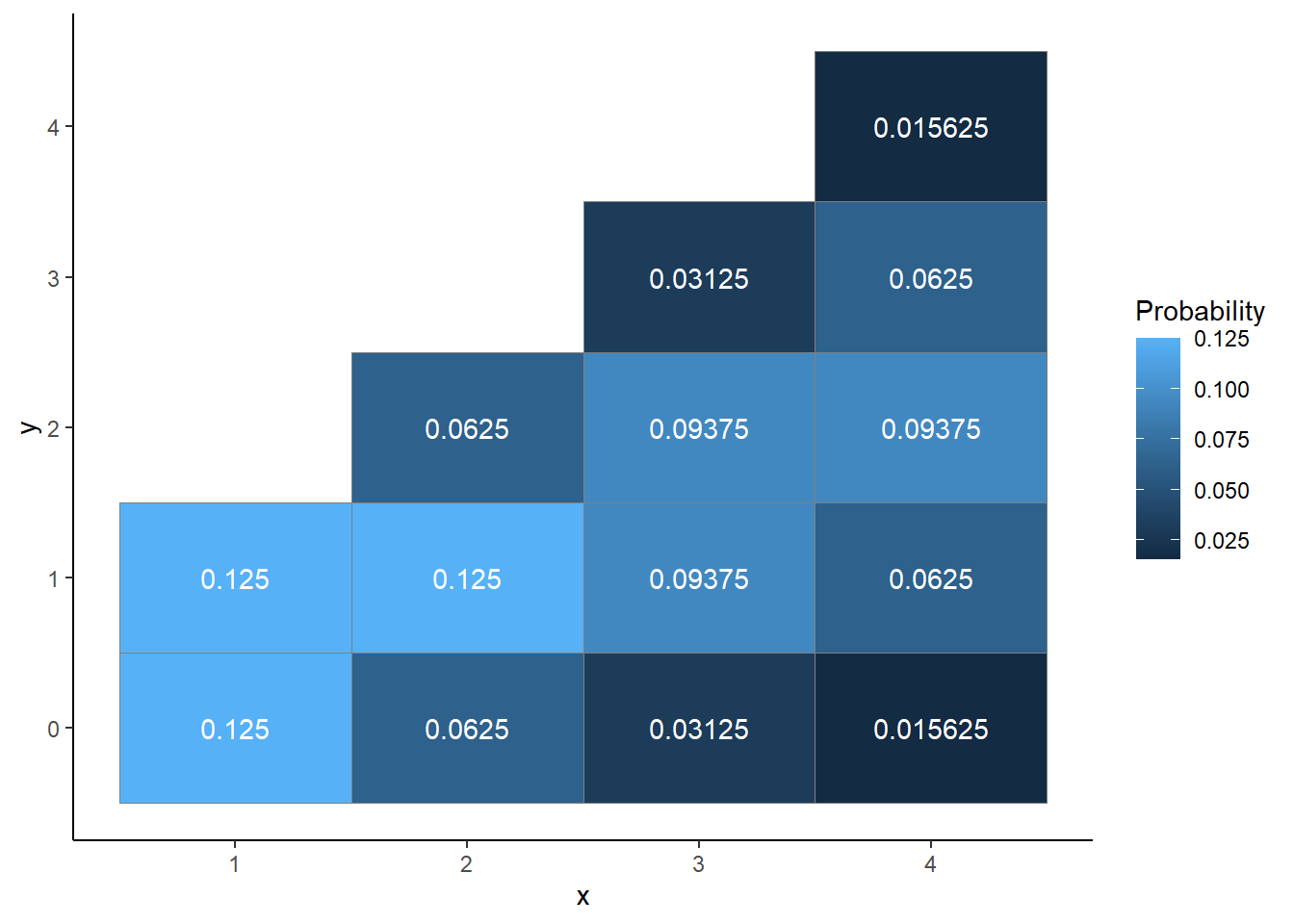
Figure 4.37: Tile plot representation of the joint distribution of \(X\) and \(Y\) in Example 4.40.

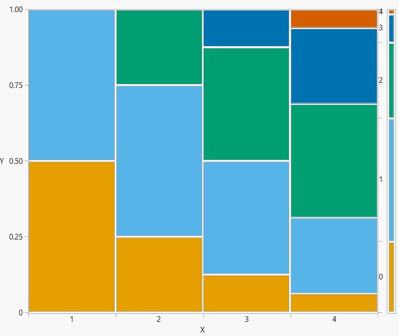
Figure 4.38: Mosaic plot representation of conditional distributions of \(Y\) given values of \(X\) in Example 4.40.

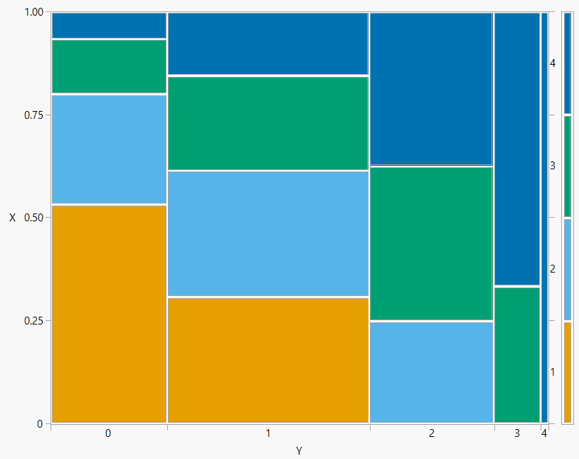
Figure 4.39: Mosaic plot representation of conditional distributions of \(X\) given values of \(Y\) in Example 4.40.

Definition 4.11 Let \(X\) and \(Y\) be two discrete random variables defined on a probability space with probability measure \(\textrm{P}\). For any fixed \(x\) with \(\textrm{P}(X=x)>0\), the conditional probability mass function (pmf) of \(Y\) given \(X=x\) is a function \(p_{Y|X}:\mathbb{R}\mapsto [0, 1]\) defined by \(p_{Y|X}(y|x)=\textrm{P}(Y=y|X=x)\). \[\begin{align*} p_{Y|X}(y|x) = \textrm{P}(Y=y|X=x) & = \frac{\textrm{P}(X=x,Y=y)}{\textrm{P}(X=x)} = \frac{p_{X,Y}(x,y)}{p_X(x)}& & \text{a function of $y$ for fixed $x$} \end{align*}\]

To emphasize, the notation \(p_{Y|X}(\cdot|x)\) represents the distribution of the random variable \(Y\) given a fixed value \(x\) of the random variable \(X\). In the expression \(p_{Y|X}(y|x)\), \(y\) is treated as the variable and \(x\) is treated like a fixed constant.

Notice that the pmfs satisfy \[ \text{conditional} = \frac{\text{joint}}{\text{marginal}} \]

Conditional distributions can be obtained from a joint distribution by slicing and renormalizing.

The conditional pmf of \(Y\) given \(X=x\) can be thought of as:

• the slice of the joint pmf \(p_{X, Y}(x, y)\) of \((X, Y)\) corresponding to \(X=x\), a function of \(y\) alone,
• renormalized — by dividing by \(p_X(x)\) — so that the probabilitiess, corresponding to different \(y\) values, for the slice sum to 1. \[ 1 = \sum_y p_{Y|X}(y|x) \quad \text{for any fixed } x \]

For a fixed \(x\), the shape of the conditional pmf of \(Y\) given \(X=x\) is determined by the shape of the \(x\)-slice of the joint pmf, \(p_{X, Y}(x, y)\). That is,

\[ \text{As a function of values of $Y$}, \quad p_{Y|X}(y|x) \propto p_{X, Y}(x, y) \]

For each fixed \(x\), the conditional pmf \(p_{Y|X}(\cdot |x)\) is a different distribution on values of the random variable \(Y\). There is not one “conditional distribution of \(Y\) given \(X\)”, but rather a family of conditional distributions of \(Y\) given different values of \(X\).

Rearranging the definition of a conditional pmf yields the multiplication rule for pmfs of discrete random variables \[\begin{align*} p_{X,Y}(x,y) & = p_{Y|X}(y|x)p_X(x)\\ & = p_{X|Y}(x|y)p_Y(y)\\ \text{joint} & = \text{conditional}\times\text{marginal} \end{align*}\]

Marginal distributions can be obtained from the joint distribution by collapsing/stacking using the law of total probability. The law of total probability for pmfs is

\[\begin{align*} p_{Y}(y) & = \sum_x p_{X,Y}(x, y)\\ & =\sum_x p_{Y|X}(y|x)p_X(x) \end{align*}\]

Bayes rule for pmfs is

\[\begin{align*} p_{X|Y}(x|y) & = \frac{p_{Y|X}(y|x)p_X(x)}{p_Y(y)} \\ p_{X|Y}(x|y) & \propto p_{Y|X}(y|x)p_X(x) \end{align*}\]

Conditioning on the value of a random variable involves treating that random variable as a constant. It is sometimes possible to identify one-way conditional distributions (\(Y\) given \(X\), or \(X\) given \(Y\)) simply by inspecting the joint pmf, without doing any calculations.

Example 4.41 \(X\) and \(Y\) are discrete random variables with joint pmf

\[ p_{X, Y} (x, y) = \frac{1}{4x}, \qquad x = 1, 2, 3, 4; y = 1, \ldots, x \]

1. Donny Dont says: “Wait, the joint pmf is supposed to be a function of both \(x\) and \(y\) but \(\frac{1}{4x}\) is only a function of \(x\).” Explain to Donny how \(p_{X, Y}\) here is, in fact, a function of both \(x\) and \(y\).
2. In which direction will it be easier to find the conditional distributions by inspection - \(Y\) given \(X\) or \(X\) given \(Y\)?
3. Without doing any calculations, find the conditional distribution of \(Y\) given \(X = 3\).
4. Without summing over the joint pmf, find the marginal probability that \(X = 3\).
5. Without doing any calculations, find a general expression for the conditional distribution of \(Y\) given \(X = x\).
6. Without summing over the joint pmf, find the marginal pmf of \(X\).
7. Describe a dice rolling scenario in which (\(X\), \(Y\)) pairs would follow this joint distribution. (Hint: you might need multiple kinds of dice.)
8. Construct a two-way table representing the joint pmf, and use it to verify your answers to the previous parts.
9. Find the marginal pmf of \(Y\). Be sure to identify the possible values.
10. Find the conditional pmf of \(X\) given \(Y=2\). Be sure to identify the possible values.

Solution. to Example 4.41

Show/hide solution

1. Don’t forget the possible values. For example, \(p_{X, Y}(3, 3) = 1/12\) but \(p_{X, Y}(3, 4) = 0\). So \(p_{X, Y}\) is a function of both \(x\) and \(y\).

2. Given \(x\), the possible values of \(Y\) are \(1, \ldots, x\). \(x\) also shows up in \(\frac{1}{4x}\) and \(y\) doesn’t. So it seems like it would be helpful to know the value of \(x\). If we treat \(x\) as a constant then we find the conditional distribution of \(Y\) given \(X=x\).

3. Treat \(X\) as the constant 3 in the joint pmf and slice to find the shape of the conditional pmf of \(Y\) given \(X=3\). \[\begin{align*} p_{Y|X} (y | 3) & \propto \frac{1}{12}, \qquad y = 1, \ldots, 3 \\ & \propto \text{constant}, \qquad y = 1, \ldots, 3 \end{align*}\] This is a distribution on \(Y\) values alone. The conditional pmf of \(Y\) given \(X=3\) is constant over its possible values, so given \(X=3\), \(Y\) is equally to be 1, 2, 3. Renormalize to get \[ p_{Y|X} (y | 3) = \frac{1}{3}, \qquad y = 1, 2, 3 \]

4. “Joint = conditional \(\times\) marginal”: \[\begin{align*} p_{X, Y}(3, y) & = p_{Y|X}(y|3)p_X(3)\\ \frac{1}{4(3)} & = \left(\frac{1}{3}\right)p_X(3) \end{align*}\] So \(p_X(3) = 1/4\). That is, \(\textrm{P}(X = 3)=1/4\).

5. We use the same process as above but with the value 3 replaced by a generic possible value \(x\). But you are still treating \(x\) as constant in the joint pmf. Slice to find the shape of the conditional pmf of \(Y\) given \(X=x\). \[\begin{align*} p_{Y|X} (y | x) & \propto \frac{1}{4x}, \qquad y = 1, \ldots, x \\ & \propto \text{constant}, \qquad y = 1, \ldots, x \end{align*}\] This is a distribution on \(Y\) values alone. Given \(x\), the possible values of \(Y\) are \(1, \ldots, x\). \(x\) is treated as constant so \(\frac{1}{4x}\) is also constant, and the conditional pmf of \(Y\) given \(X=x\) is constant over its possible values. That is, given \(X=x\), \(Y\) is equally to be \(1, \ldots, x\). Renormalize — each of the \(x\) equally likely values of \(Y\) occurs with probability \(1/x\) — to get \[ p_{Y|X} (y | x) = \frac{1}{x}, \qquad y = 1, \ldots, x \]

6. “Joint = conditional \(\times\) marginal”. For \(x = 1, 2, 3, 4\): \[\begin{align*} p_{X, Y}(x, y) & = p_{Y|X}(y|x)p_X(x)\\ \frac{1}{4x} & = \left(\frac{1}{x}\right)p_X(x) \end{align*}\] So \(p_X(x) = 1/4, x = 1, 2, 3, 4\). That is, \(X\) is equally like to be 1, 2, 3, 4.

7. Roll a fair four-sided die once and let \(X\) be the result. Then, given \(X=x\), roll a fair “\(x\)-sided die”¹²⁰ once and let \(Y\) be the result.

8. See the table below. Note that we can also write the possible pairs as: \(y = 1, 2, 3, 4; x = y, \ldots, 4\).

   \(p_{X, Y}(x, y)\)
   \(x\) \ \(y\)	1	2	3	4	\(p_{X}(x)\)
   1	12/48	0	0	0	1/4
   2	6/48	6/48	0	0	1/4
   3	4/48	4/48	4/48	0	1/4
   4	3/48	3/48	3/48	3/48	1/4
   \(p_Y(y)\)	25/48	13/48	7/38	3/48

9. Marginally, the possible values of \(Y\) are 1, 2, 3, 4. The marginal pmf of \(Y\) is a function of \(y\) alone, but there is no simple closed form expression in this case.

   \(y\)	\(p_Y(y)\)
   1	25/48
   2	13/48
   3	7/48
   4	3/48

10. Given \(Y=2\), \(X\) takes possible values 2, 3, 4. Slice the column of the joint pmf table corresponding to \(Y=2\) and renormalize. Given \(Y=2\), \(X\) is two times more likely to be 2 than to be 4, and \(X\) is 1.5 times more likely to be 2 than to be 3. The conditional pmf of \(X\) given \(Y=2\) is a distribution of values of \(X\) alone, treating \(Y=2\) as constant.

    \(x\)	\(p_{X|Y}(x|2)\)
    2	6/13
    3	4/13
    4	3/13

The code below defines a custom probability space corresponding to the two-stage conditional simulation in the previous example, and then defines random variables on this probability space.

def conditional_dice():
  x = DiscreteUniform(1, 4).draw()
  if x == 1:
    y = 1
  else:
    y = DiscreteUniform(1, x).draw()
  return x, y

X, Y = RV(ProbabilitySpace(conditional_dice))

(X & Y).sim(10000).plot('tile')

Y.sim(10000).plot()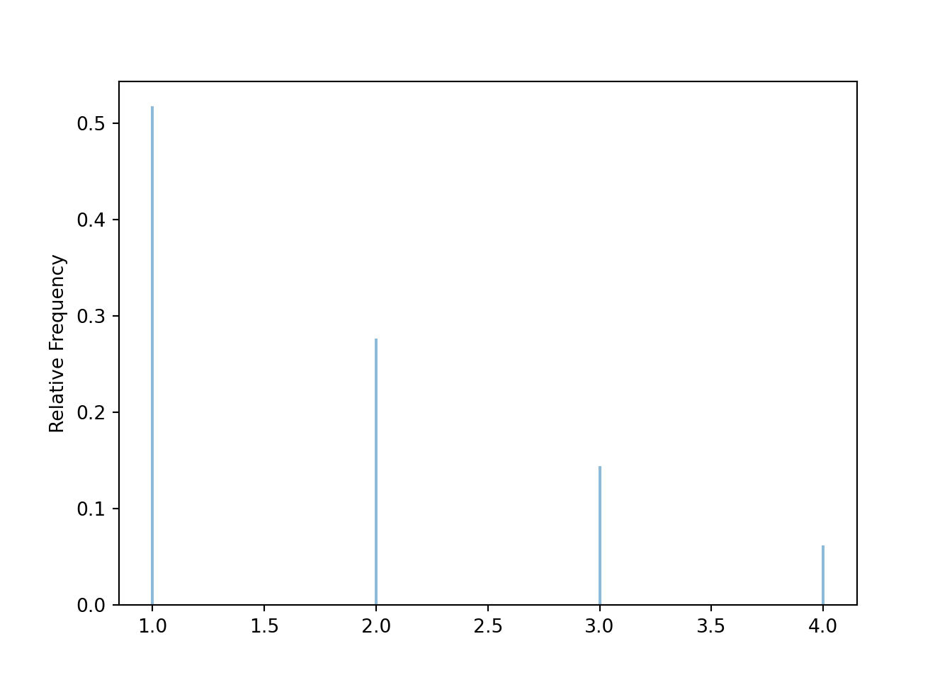

(X | (Y == 2) ).sim(10000).plot()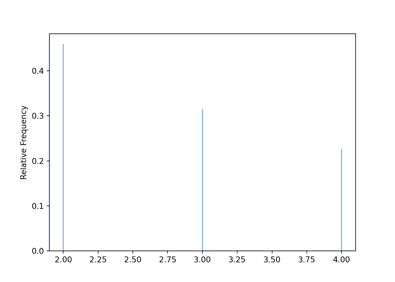

Be sure to distinguish between joint, conditional, and marginal distributions.

• The joint distribution is a distribution on \((X, Y)\) pairs. A mathematical expression of a joint distribution is a function of both values of \(X\) and values of \(Y\). In particular, the joint pmf \(p_{X, Y}\) is a function of both values of \(X\) and values of \(Y\). Pay special attention to the possible values; the possible values of one variable might be restricted by the value of the other.
• The conditional distribution of \(Y\) given \(X=x\) is a distribution on \(Y\) values (among \((X, Y)\) pairs with a fixed value of \(X=x\)). A mathematical expression of a conditional distribution will involve both \(x\) and \(y\), but \(x\) is treated like a fixed constant and \(y\) is treated as the variable. In particular, the conditional pmf \(p_{Y|X}\) is a function of values of \(Y\) for a fixed value of \(x\); treat \(x\) like a constant and \(y\) as the variable. Note: the possible values of \(Y\) might depend on the value of \(x\), but \(x\) is treated like a constant.
• The marginal distribution of \(Y\) is a distribution on \(Y\) values only, regardless of the value of \(X\). A mathematical expression of a marginal distribution will have only values of the single variable in it; for example, an expression for the marginal distribution of \(Y\) will only have \(y\) in it (no \(x\), not even in the possible values). In particular, the marginal pmf \(p_Y\) is a function of values of \(Y\) only.

4.8.2 Continuous random variables: Conditional probability density functions

Remember that continuous random variables are described by probability density functions which can be integrated to find probabilities.

Bivariate Normal distributions are one commonly used family of joint continuous distribution. For example, the following plots represent the joint pdf surface of the Bivariate Normal distribution in the meeting problem in Section 2.12.1, with correlation 0.7. In \(X\) and \(Y\) have a Bivariate Normal distribution, then the conditional distribution of \(X\) given any value of \(Y\) is a Normal distribution (likewise for \(Y\) given any value of \(X\).)

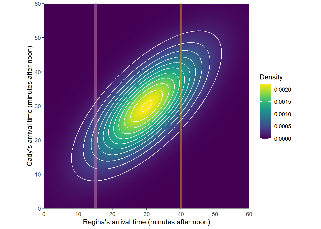
Figure 4.40: A Bivariate Normal distribution with two \(X\)-slices highlighted.

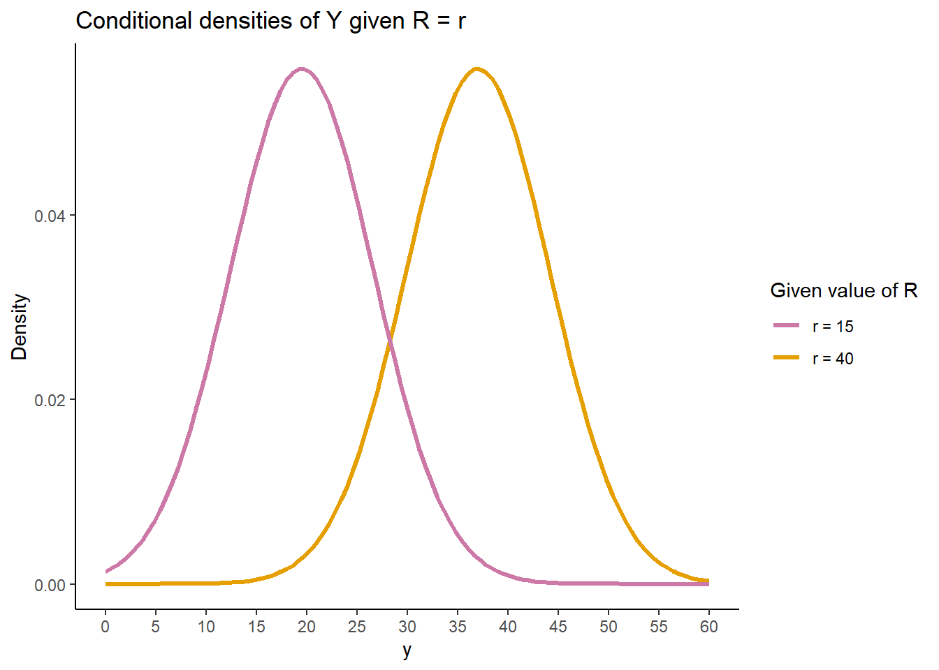
Figure 4.41: Conditional distributions of \(Y\) given \(X=x\) for the two \(x\)-slices in Figure 4.40.

Definition 4.12 Let \(X\) and \(Y\) be two continuous random variables with joint pdf \(f_{X,Y}\) and marginal pdfs \(f_X, f_Y\). For any fixed \(x\) with \(f_X(x)>0\), the conditional probability density function (pdf) of \(Y\) given \(X=x\) is a function \(f_{Y|X}:\mathbb{R}\mapsto [0, \infty)\) defined by \[\begin{align*} f_{Y|X}(y|x) &= \frac{f_{X,Y}(x,y)}{f_X(x)}& & \text{a function of $y$ for fixed $x$} \end{align*}\]

To emphasize, the notation \(f_{Y|X}(y|x)\) represents a conditional distribution of the random variable \(Y\) for a fixed value \(x\) of the random variable \(X\). In the expression \(f_{Y|X}(y|x)\), \(x\) is treated like a constant and \(y\) is treated as the variable.

Notice that the pdfs satisfy \[ \text{conditional} = \frac{\text{joint}}{\text{marginal}} \]

Conditional distributions can be obtained from a joint distribution by slicing and renormalizing.

The conditional pdf of \(Y\) given \(X=x\) can be thought of as:

• the slice of the joint pdf \(f_{X, Y}(x, y)\) of \((X, Y)\) corresponding to \(X=x\), a function of \(y\) alone,
• renormalized — by dividing by \(f_X(x)\) — so that the density heights, corresponding to different \(y\) values, for the slice are such that the total area under the density slice is 1. \[ 1 = \int_{-\infty}^\infty f_{Y|X}(y|x)\, dy \quad \text{for any fixed } x \]

For a fixed \(x\), the shape of the conditional pdf of \(Y\) given \(X=x\) is determined by the shape of the \(x\)-slice of the joint pdf, \(f_{X, Y}(x, y)\). That is,

\[ \text{As a function of values of $Y$}, \quad f_{Y|X}(y|x) \propto f_{X, Y}(x, y) \]

For each fixed \(x\), the conditional pdf \(f_{Y|X}(\cdot |x)\) is a different distribution on values of the random variable \(Y\). There is not one “conditional distribution of \(Y\) given \(X\)”, but rather a family of conditional distributions of \(Y\) given different values of \(X\).

Rearranging the definition of a conditional pdf yields the multiplication rule for pdfs of continuous random variables \[\begin{align*} f_{X,Y}(x,y) & = f_{Y|X}(y|x)f_X(x)\\ & = f_{X|Y}(x|y)f_Y(y)\\ \text{joint} & = \text{conditional}\times\text{marginal} \end{align*}\]

Marginal distributions can be obtained from the joint distribution by collapsing/stacking using the law of total probability. The law of total probability for pdfs is

\[\begin{align*} f_{Y}(y) & = \int_{-\infty}^\infty f_{X,Y}(x, y)\, dx\\ & =\int_{-\infty}^\infty f_{Y|X}(y|x)f_X(x)\, dx \end{align*}\]

Bayes rule for pdfs is

\[\begin{align*} f_{X|Y}(x|y) & = \frac{f_{Y|X}(y|x)f_X(x)}{f_Y(y)} \\ f_{X|Y}(x|y) & \propto f_{Y|X}(y|x)f_X(x) \end{align*}\]

Example 4.42 Recall Example 4.36. Consider the probability space corresponding to two spins of the Uniform(1, 4) spinner and let \(X\) be the sum of the two spins and \(Y\) the larger to the two spins (or the common value if a tie). Recall that the joint pdf is \[ f_{X, Y}(x, y) = \begin{cases} 2/9, & 2<x<8,\; 1<y<4,\; x/2<y<x-1,\\ 0, & \text{otherwise,} \end{cases} \] the marginal pdf of \(Y\) is \[ f_Y(y) = \begin{cases} (2/9)(y-1), & 1<y<4,\\ 0, & \text{otherwise,} \end{cases} \] and the marginal pdf of \(X\) is \[ f_X(x) = \begin{cases} (1/9)(x-2), & 2 < x< 5,\\ (1/9)(8-x), & 5<x<8,\\ 0, & \text{otherwise.} \end{cases} \]

1. Find \(f_{X|Y}(\cdot|3)\), the conditional pdf of \(X\) given \(Y=3\).
2. Find \(\textrm{P}(X > 5.5 | Y = 3)\).
3. Find \(f_{X|Y}(\cdot|4)\), the conditional pdf of \(X\) given \(Y=4\).
4. Find \(\textrm{P}(X > 5.5 | Y = 4)\).
5. Find \(f_{X|Y}(\cdot|y)\), the conditional pdf of \(X\) given \(Y=y\), for \(1<y<4\).
6. Find \(f_{Y|X}(\cdot|3.5)\), the conditional pdf of \(Y\) given \(x=3.5\).
7. Find \(f_{Y|X}(\cdot|6)\), the conditional pdf of \(Y\) given \(x=6\).
8. Find \(f_{Y|X}(\cdot|x)\), the conditional pdf of \(Y\) given \(x\).

Solution. to Example 4.42

Show/hide solution

1. See the top left plot of Figure 4.42; the conditional pdf corresponds to the renormalized slice of the joint pdf along \(Y=3\). If \(Y=3\) then \(X\) takes values between 4 and 6, and the density is constant over this interval of length 2. \[ f_{X|Y}(x| 3) = \begin{cases} \frac{1}{2}, & 4 < x < 6,\\ 0, & \text{otherwise.} \end{cases} \] We could also use “conditional is joint divided by marginal”. The marginal density of \(Y\) at \(y=3\) is \(f_Y(3) = (2/9)(3-1) = 4/9\). For the slice of the joint pdf along \(y=3\), be careful to note that \(f_{X, Y}(x, 3)=2/9\) only if \(4<x<6\) and \(f_{X, Y}(x, 3) = 0\) for \(x\) outside of this range. \[ f_{X|Y}(x| 3) = \frac{f_{X, Y}(x, 3)}{f_Y(3)} = \begin{cases} \frac{2/9}{4/9}, & 4 < x< 6\\ 0, & \text{otherwise.} \end{cases} \]
2. Use the conditional pdf of \(X\) given \(Y=3\) to compute \(\textrm{P}(X > 5.5 | Y = 3)\). Since the conditional pdf is Uniform(4, 6), the probability should just be \((6-5.5)/(6-4) = 0.25\). To compute Via integration, note we integrate over values of \(X\) \[ \textrm{P}(X > 5.5 | Y = 3) = \int_{5.5}^6 \frac{1}{2}dx = \frac{x}{2}\Bigg|_{x=5.5}^{x=6} = 0.25 \]
3. See the top right plot of Figure 4.42; the conditional pdf corresponds to the renormalized slice of the joint pdf along \(Y=4\). If \(Y=4\) then \(X\) takes values between 5 and 8, and the density is constant over this interval of length 3. \[ f_{X|Y}(x| 3) = \begin{cases} \frac{1}{3}, & 5 < x < 8,\\ 0, & \text{otherwise.} \end{cases} \]
4. Use the conditional pdf of \(X\) given \(Y=4\) to compute \(\textrm{P}(X > 5.5 | Y = 4)\). Since the conditional pdf is Uniform(5, 8), the probability should just be \((8-5.5)/(8-5) = 5/6\). Via integration; note we integrate over values of \(X\) \[ \textrm{P}(X > 5.5 | Y = 4) = \int_{5.5}^8 \frac{1}{3}dx = \frac{x}{3}\Bigg|_{x=5.5}^{x=8} = 5/6 \]
5. Treat \(y\) as a constant, like in the previous parts. The conditional pdf corresponds to the renormalized slice of the joint pdf along \(Y=y\). If \(Y=y\) then \(X\) takes values between \(y+1\) and \(2y\), and the density is constant over this interval of length \(2y - (y +1) = y - 1\). \[ f_{X|Y}(x| y) = \begin{cases} \frac{1}{y-1}, & y+1 < x < 2y,\\ 0, & \text{otherwise.} \end{cases} \] We could also use “conditional is joint divided by marginal”. The marginal density of \(Y\) at \(y\) is \(f_Y(y) = (2/9)(y-1)\). For the slice of the joint pdf along \(y\), be careful to note that \(f_{X, Y}(x, y)=2/9\) only if \(y+1<x<2y\) and \(f_{X, Y}(x, y) = 0\) for \(x\) outside of this range. \[ f_{X|Y}(x| y) = \frac{f_{X, Y}(x, y)}{f_Y(y)} = \begin{cases} \frac{2/9}{2/9(y-1)}, & y+1 < x< 2y\\ 0, & \text{otherwise.} \end{cases} \] Remember, we are treating \(y\) as given and fixed. The conditional pdf of \(X\) given \(Y=y\) is a density on values of \(X\).
6. See the bottom left plot of Figure 4.42; the conditional pdf corresponds to the renormalized slice of the joint pdf along \(X=3.5\). If \(X=3.5\) then \(Y\) takes values between 1.75 and 2.5, and the density is constant over this interval of length 0.75. \[ f_{Y|X}(y| 4) = \begin{cases} \frac{1}{0.75}, & 1.75 < y < 2.5,\\ 0, & \text{otherwise.} \end{cases} \] We could also use “conditional is joint divided by marginal”. The marginal density of \(X\) at \(x=3.5\) is \(f_X(3.5) = (1/9)(3.5-2) = 1.5/9\). For the slice of the joint pdf along \(x=3.5\), be careful to note that \(f_{X, Y}(3.5, y)=2/9\) only if \(1.75< y <2.5\) and \(f_{X, Y}(3.5, y) = 0\) for \(y\) outside of this range. \[ f_{Y|X}(y| 3.5) = \frac{f_{X, Y}(3.5, y)}{f_X(3.5)} = \begin{cases} \frac{2/9}{1.5/9}, & 1.75 < y< 2.5\\ 0, & \text{otherwise.} \end{cases} \]
7. See the bottom right plot of Figure 4.42; the conditional pdf corresponds to the renormalized slice of the joint pdf along \(X=6\). If \(X=6\) then \(Y\) takes values between 3 and 4, and the density is constant over this interval of length 1. \[ f_{Y|X}(y| 6) = \begin{cases} 1, & 3 < y < 4,\\ 0, & \text{otherwise.} \end{cases} \]
8. There are two general cases. If \(2<x<5\) then \(Y\) takes values between \(0.5x\) and \(x-1\), and \(f_X(x) = (1/9)(x-2)\). If \(5<x<8\) then \(Y\) takes values between \(0.5x\) and \(4\), and \(f_X(x) = (1/9)(8-x)\). \[ f_{Y|X}(y| x) = \frac{f_{X, Y}(x, y)}{f_X(x)} = \begin{cases} \frac{2/9}{(1/9)(x-2)}, & 2<x<5, 0.5x< y< x-1\\ \frac{2/9}{(1/9)(8-x)}, & 5<x<8, 0.5x< y< 4\\ 0, & \text{otherwise.} \end{cases} \] Therefore, \[ f_{Y|X}(y| x) = \begin{cases} \frac{1}{0.5x - 1}, & 2<x<5, 0.5x< y< x-1\\ \frac{1}{4 - 0.5x}, & 5<x<8, 0.5x< y< 4\\ 0, & \text{otherwise.} \end{cases} \] Even though the above expression involves both \(x\) and \(y\), we are treating \(x\) as fixed as \(y\) as the variable. For a given \(x\), the conditional pdf of \(Y\) given \(X=x\) is a density of values of \(Y\) only.

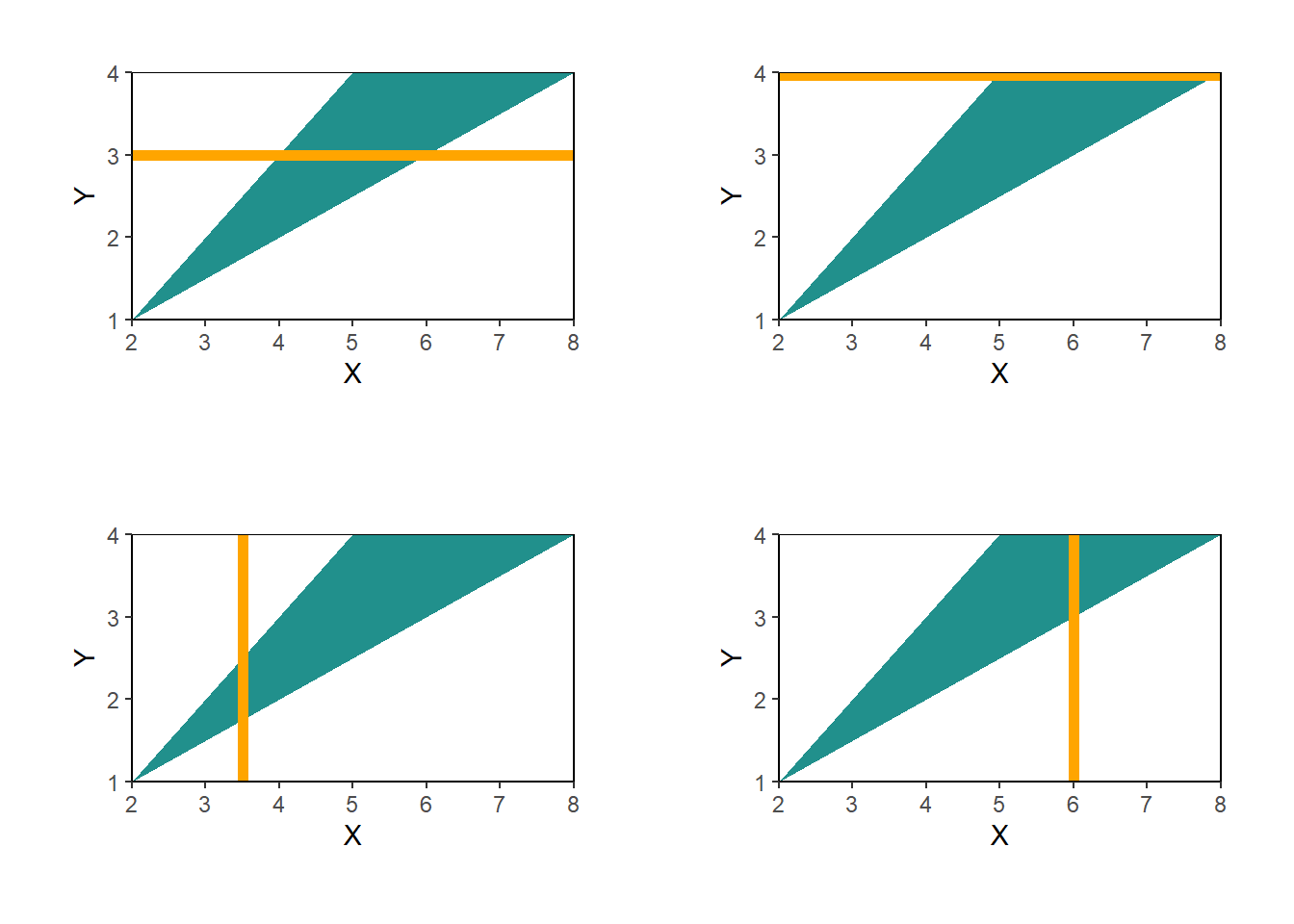
Figure 4.42: Illustration of the joint pdf and conditional pdfs in Example 4.42.

The conditional pdf of \(Y\) given \(X=x\) can be integrated to find conditional probabilities of events involving \(Y\) given \(X=x\).
\[\begin{align*} \textrm{P}(a \le Y \le b \vert X = x) & =\int_a^b f_{Y|X}(y|x) dy, \qquad \text{for all } -\infty \le a \le b \le \infty \end{align*}\] In the above, \(x\) is treated as fixed and \(y\) as the variable being integrated over. The resulting probability \(\textrm{P}(a<Y<b|X=x)\) will be a function of \(x\). For a given \(x\), \(\textrm{P}(a<Y<b|X=x)\) is a single number.

Be careful when conditioning with continuous random variables. Remember to specify possible values! And to note how conditioning can change the possible values.

Example 4.43 Donny Don’t writes the following Symbulate code approximate the conditional distribution of \(X\) given \(Y=3\) in Example 4.42. What do you think will happen when Donny runs his code?

P = (Uniform(0, 1) ** 2)

X = RV(P, sum)

Y = RV(P, max)

(X | (Y == 3) ).sim(10000)

Solution. to Example 4.43

Show/hide solution

Donny’s code will run forever! Remember, \(Y\) is a continuous random variable, so \(\textrm{P}(Y = 3)=0\). The simulation will never return a single value of \(Y\) equal to \(3.0000000\ldots\), let alone 10000 of them.

Be careful when conditioning with continuous random variables. Remember that the probability that a continuous random variable is equal to a particular value is 0; that is, for continuous \(X\), \(\textrm{P}(X=x)=0\). When we condition on \(\{X=x\}\) we are really conditioning on \(\{|X-x|<\epsilon\}\) and seeing what happens in the idealized limit when \(\epsilon\to0\).

When simulating, never condition on \(\{X=x\}\); rather, condition on \(\{|X-x|<\epsilon\}\) where \(\epsilon\) represents some suitable degree of precision (e.g. \(\epsilon=0.005\) if rounding to two decimal places).

Remember pdfs do not return probabilities directly; \(f_{Y|X}(y|x)\) is not a probability of anything. But \(f_{Y|X}(y|x)\) is related to the probability that \(Y\) is “close to” \(y\) given that \(X\) is “close to” \(x\): \[ \textrm{P}(y-\epsilon/2<Y < y+\epsilon/2\; \vert\; x-\epsilon/2<X < x+\epsilon/2) \approx \epsilon f_{Y|X}(y|x) \]

The code below approximates conditioning on the event \(\{Y = 3\}\) by conditioning instead on the event that \(Y\) rounded to the nearest tenth is equal to 3, \(\{|Y - 3| < 0.05\} = \{2.95<Y<3.05\}\).

U1, U2 = RV(Uniform(1, 4) ** 2)

X = U1 + U2

Y = (U1 & U2).apply(max)

( (X & Y) | (abs(Y - 3) < 0.01) ).sim(10)

Index	Result
0	(5.193607575852882, 3.0015240675845107)
1	(4.551611258791802, 2.998528076122441)
2	(4.137168248043998, 3.0099625542286987)
3	(5.023000224381788, 3.0046509020963192)
4	(5.66888285214946, 3.000717270531224)
5	(4.160204452188206, 3.0027986349173066)
6	(5.452801800774074, 2.9975960580389627)
7	(5.866466312395542, 2.9938130119921773)
8	(5.173903944796324, 2.9929770679718577)
...	...
9	(4.198846670510781, 3.007317317674553)

The code below simulates the approximate conditional distribution of \(X\) given \(Y=3\). The event \(\{|Y - 3|<0.05\}\) has approximate probability \(0.1f_Y(3) = 0.1(4/9)=0.044\). In order to obtain 10000 repetitions for which the event \(\{|Y - 3|<0.05\}\), we would have to run around 225,000 repetitions in total.

plt.figure()
( X | (abs(Y - 3) < 0.05) ).sim(10000).plot()
plt.show()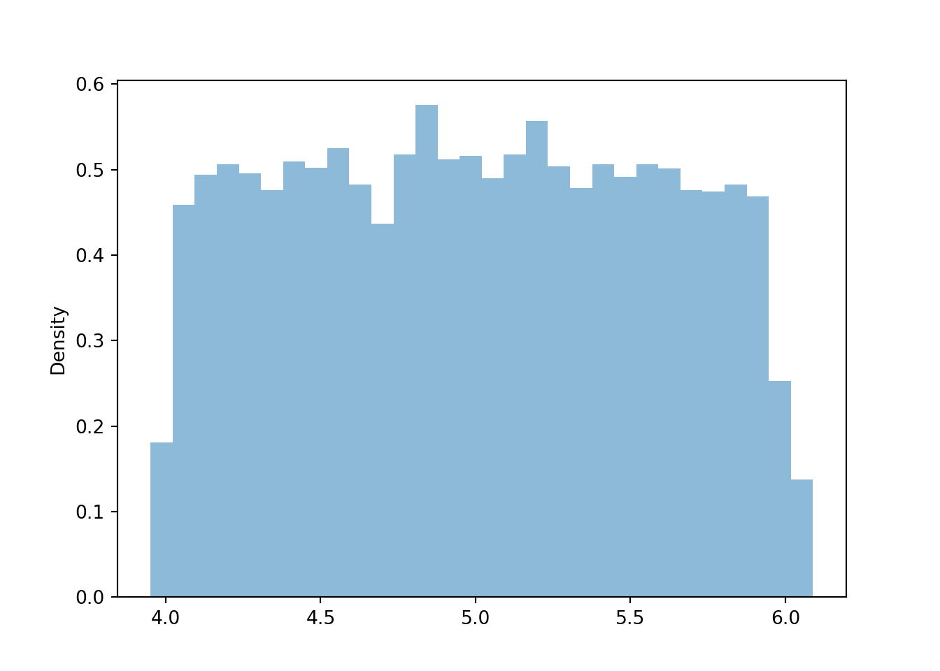

Given a joint pdf \(f_{X, Y}\), it is sometimes possible to identify the conditional pdfs in one direction just by inspection. Remember that the conditional pdf of \(Y\) given \(X=x\) is a distribution of values of \(Y\) alone. Therefore, treat \(x\) as fixed and view \(f_{X, Y}\) as a function of \(y\) alone; is the resulting function a recognizable pdf? By “recognizable” we mean is it among a common named family of distributions like Uniform, Exponential, Normal, etc. If the conditional pdf \(f_{Y|X}\) can be identified, then the marginal pdf \(f_X\) can be found without any calculus. If fixing \(x\) does not lead to a recognizable pdf, try fixing \(y\) instead.

Example 4.44 Suppose \(X\) and \(Y\) are continuous RVs with joint pdf \[ f_{X, Y}(x, y) = \frac{1}{x}e^{-x}, \qquad x > 0,\quad 0<y<x. \]

1. Donny Dont says: “Wait, the joint pdf is supposed to be a function of both \(x\) and \(y\) but \(\frac{1}{x}e^{-x}\) is only a function of \(x\).” Explain to Donny how \(f_{X, Y}\) here is, in fact, a function of both \(x\) and \(y\).
2. Identify by name the one-way conditional distributions that you can obtain from the joint pdf (without doing any calculus or computation).
3. Identify by name the marginal distribution you can obtain without doing any calculus or computation.
4. Describe how could you use the Exponential(1) spinner and the Uniform(0, 1) spinner to generate an \((X, Y)\) pair.
5. Sketch a plot of the joint pdf.
6. Sketch a plot of the marginal pdf of \(Y\).
7. Set up the calculation you would perform to find the marginal pdf of \(Y\).

Solution. to Example 4.44

Show/hide solution

1. Don’t forget the possible values. For example, \(f_{X, Y}(1, 0.5) = e^{-1}\) but \(f_{X, Y}(1, 2) = 0\). So \(f_{X, Y}\) is a function of both \(x\) and \(y\).

2. Since \(x\) shows up in more places, try conditioning on \(x\) first and treat it as fixed. If \(x\) is treated as constant, then \(\frac{1}{x}e^{-x}\) is also treated as constant. The conditional density of \(Y\) given \(X=x\), as a function of \(y\) has the form \[ f_{Y|X}(y|x) \propto \text{constant}, \quad 0<y<x \] The height along the \(x\) slice is constant as a function of \(y\), but don’t forget to include the possible values. That is, the conditional pdf of \(Y\) is constant for values of \(y\) between 0 and \(x\) (and 0 otherwise). Therefore, given \(X=x\) the conditional distribution of \(Y\) is the Uniform(0, \(x\)) distribution. Now we just we need to fill in the correct constant that makes the density integrate to 1.
   \[ f_{Y|X}(y|x) = \frac{1}{x}, \quad 0<y<x \] Remember this is a density on values of \(Y\) with \(x\) fixed.
   

3. Since we have the joint pdf and the conditional pdfs of \(Y\) given each value of \(X\), we can find the marginal pdf of \(X\). For possible \((x, y)\) pairs \[\begin{align*} \text{Joint} & = \text{Conditional}\times \text{Marginal}\\ f_{X, Y}(x, y) & = f_{Y|X}(y|x)f_X(x) \\ \frac{1}{x}e^{-x} & = \left(\frac{1}{x}\right) f_X(x) \end{align*}\] Therefore \[ f_X(x) = e^{-x}, \qquad x>0 \] That is, the marginal distribution of \(X\) is the Exponential(1) distribution.

4. Spin the Exponential(1) spinner to generate \(X\). Then, given \(X=x\), spin the Uniform(0, \(x\)) spinner to generate \(Y\). For example, if \(X=2\) we want to generate \(Y\) from a Uniform(0, 2) distribution. Remember that we can generate values from any Uniform distribution by generating a value from a Uniform(0, 1) distribution and then applying an appropriate linear rescaling. Spin the Uniform(0, 1) spinner to generate \(U\), and let \(Y=XU\). For example, if \(X=2\) then \(Y=2U\) follows a Uniform(0, 2) distribution. In summary,

   • Spin the Exponential(1) spinner once and let \(X\) be the result
   • Spin the Uniform(0, 1) spinner once and let \(U\) be the result
   • Let \(Y = XU\).

5. See the simulation output below for an illustration. Start by sketching \(X\) values; the density will be highest near 0 and decrease as \(x\) increases. Then, for each value of \(x\) sketch \(y\) values uniformly between 0 and \(x\).

6. Overall, \(Y\) can take any positive value \(y>0\). For each \(y\), collapse the joint pdf over all \(x\) values. The density will be highest at \(y=0\) and then decrease as \(y\) increases.

7. We can find the marginal pdf of \(Y\) by integrating out the \(x\)’s in the joint pdf. Remember that the joint pdf is 0 unless \(y<x\). For \(y>0\), \[\begin{align*} f_Y(y) & = \int_{y}^\infty \frac{1}{x}e^{-x} \, dx \end{align*}\] There is no simple closed form expression, but it is a function of \(y\) alone, for \(y>0\); the \(x\)’s have been integrated out.

X, U = RV(Exponential(1) * Uniform(0, 1))

Y = X * U

plt.figure()
(X & Y).sim(1000).plot()
plt.show()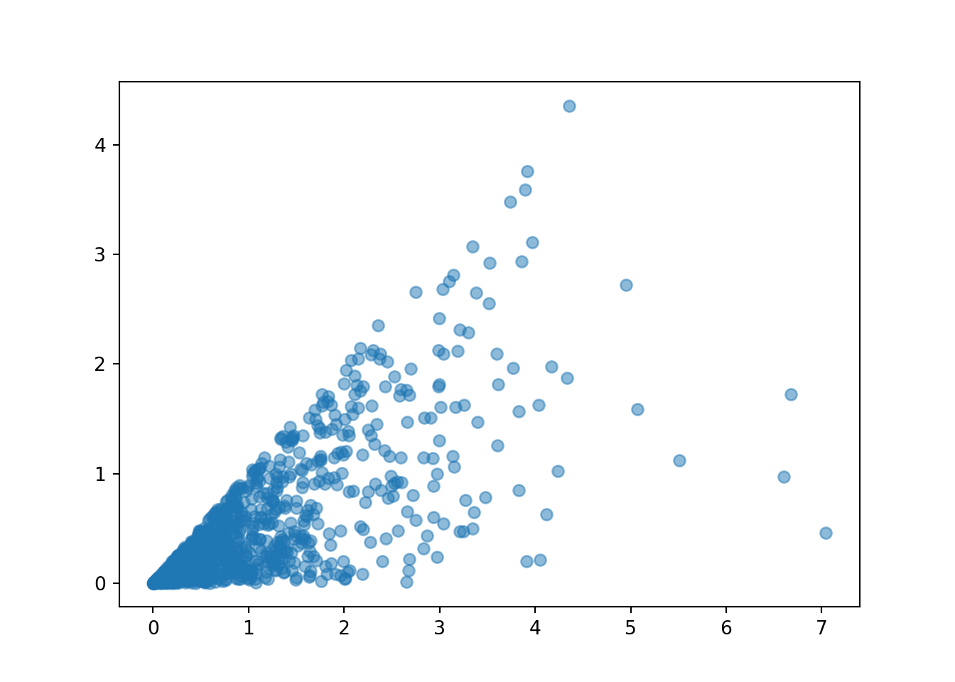

plt.figure()
Y.sim(10000).plot()
plt.show()

Be sure to distinguish between joint, conditional, and marginal distributions.

• The joint distribution is a distribution on \((X, Y)\) pairs. A mathematical expression of a joint distribution is a function of both values of \(X\) and values of \(Y\). In particular, a joint pdf \(f_{X, Y}\) is a function of both values of \(X\) and values of \(Y\). Pay special attention to the possible values; the possible values of one variable might be restricted by the value of the other.
• The conditional distribution of \(Y\) given \(X=x\) is a distribution on \(Y\) values (among \((X, Y)\) pairs with a fixed value of \(X=x\)). A mathematical expression of a conditional distribution will involve both \(x\) and \(y\), but \(x\) is treated like a fixed constant and \(y\) is treated as the variable. In particular, a conditional pdf \(f_{Y|X}\) is a function of values of \(Y\) for a fixed value of \(x\); treat \(x\) like a constant and \(y\) as the variable. Note: the possible values of \(Y\) might depend on the value of \(x\), but \(x\) is treated like a constant.
• The marginal distribution of \(Y\) is a distribution on \(Y\) values only, regardless of the value of \(X\). A mathematical expression of a marginal distribution will have only values of the single variable in it; for example, an expression for the marginal distribution of \(Y\) will only have \(y\) in it (no \(x\), not even in the possible values). In particular, a marginal pdf \(f_Y\) is a function of values of \(Y\) only.

---

119. We mostly focus on the case of two random variables, but analogous definitions and concepts apply for more than two (though the notation can get a bit messier).↩︎

120. A “one-sided” die always returns 1. A “two-sided” die could be a coin with heads labeled 1 and tails labeled 2. A “three-sided” die could be a six-sided die with two sides each labeled 1, 2, 3.↩︎