2.13 Conditional distributions

The joint distribution of random variables $X$ and $Y$ (defined on the same probability space) is a probability distribution on $(x, y)$ pairs, and describes how the values of $X$ and $Y$ vary together or jointly. We can also study conditional distributions of random variables given the values of some random variables. How does the distribution of $Y$ change for different values of $X$ (and vice versa)?

2.13.1 Conditional distributions of discrete random variables

Example 2.59 Roll a fair four-sided die twice. Let $X$ be the sum of the two rolls, and let $Y$ be the larger of the two rolls (or the common value if a tie). We have previously found the joint and marginal distributions of $X$ and $Y$, displayed in the two-way table below.

$(x, y)$
	1	2	3	4	Total
2	1/16	0	0	0	1/16
3	0	2/16	0	0	2/16
4	0	1/16	2/16	0	3/16
5	0	0	2/16	2/16	4/16
6	0	0	1/16	2/16	3/16
7	0	0	0	2/16	2/16
8	0	0	0	1/16	1/16
Total	1/16	3/16	5/16	7/16

Compute $\textrm{P}(X=6|Y=4)$.
Construct a table, plot, and spinner to represent the conditional distribution of $X$ given $Y=4$.
Construct a table, plot, and spinner to represent the conditional distribution of $X$ given $Y=3$.
Construct a table, plot, and spinner to represent the conditional distribution of $X$ given $Y=2$.
Construct a table, plot, and spinner to represent the conditional distribution of $X$ given $Y=1$.
Compute $\textrm{P}(Y=4|X=6)$.
Construct a table, plot, and spinner to represent the distribution of $Y$ given $X=6$.
Construct a table, plot, and spinner to represent the distribution of $Y$ given $X=5$.
Construct a table, plot, and spinner to represent the distribution of $Y$ given $X=4$.

Solution. to Example 2.59

Show/hide solution

Remember that $\{X=6\}$ and $\{Y=4\}$ are events, so we use the definition of conditional probability for events. \[ \textrm{P}(X = 6 | Y = 4) =\frac{\textrm{P}(X = 6, Y = 4)}{\textrm{P}(Y=4)} = \frac{2/16}{7/16} = 2/7 \]
Slice the column of the joint distribution table corresponding to $Y=4$, and then renormalize. If $Y = 4$ then $X$ is either 5, 6, 7, or 8; $Y$ is equally likely to be 5, 6, or 7, and each of those values is twice as likely as 8. The table below displays the conditional distribution of $X$ given $Y=4$. (See further down for plots and spinners.) Note well that this is a distribution of values of $X$.

$x$ $\textrm{P}(X = x|Y = 4)$

5 2/7

6 2/7

7 2/7

8 1/7
Slice the column of the joint distribution table corresponding to $Y=3$, and then renormalize. Given $Y=3$, $X$ is equally likely to be either 4 or 5, and each of those values is twice as likely as 6. Note that changing the condition from $\{Y=4\}$ to $\{Y=3\}$ changes the possible values of $X$, along with their probabilities.

$x$ $\textrm{P}(X = x | Y = 3)$

4 2/5

5 2/5

6 1/5
Slice the column of the joint distribution table corresponding to $Y=3$, and then renormalize. Given $Y=2$, $X$ is twice as likely to be 3 than 4.

$x$ $\textrm{P}(X = x | Y = 2)$

3 2/3

4 1/3
Given $Y=1$, $X$ is equal to 2 with probability 1: $\textrm{P}(X = 2 | Y = 1)=1$.
Remember that $\textrm{P}(X = 6 | Y = 4)$ and $\textrm{P}(Y = 4 | X = 6)$ measure different probabilities. \[ \textrm{P}(Y = 4 | X = 6) =\frac{\textrm{P}(X = 6, Y = 4)}{\textrm{P}(X=6)} = \frac{2/16}{3/16} = 2/3 \]
Slice the row of the joint distribution table corresponding to $X=6$, and then renormalize. If $X = 6$ then $Y$ is either 3 or 4, and $Y$ is twice as likely to be 4 than 3. The table below represents the conditional distribution of $Y$ given $X = 6$. Note that this is a distribution of $Y$ values.

$y$ $\textrm{P}(Y = y | X = 6)$

3 1/3

4 2/3
Slice the row of the joint distribution table corresponding to $X=5$, and then renormalize. If $X=5$ then $Y$ is equally likely to be 3 or 4.

$y$ $\textrm{P}(Y = y | X = 5)$

3 1/2

4 1/2
Slice the row of the joint distribution table corresponding to $X=4$, and then renormalize. If $X=4$ then $Y$ is twice as likely to be 3 than 2. Note that changing the condition from $\{X=5\}$ to $\{X=4\}$ changes the possible values of $Y$, along with their probabilities.

$y$ $\textrm{P}(Y = y | X = 5)$

2 1/3

3 2/3

\(x\)	\(\textrm{P}(X = x\|Y = 4)\)
5	2/7
6	2/7
7	2/7
8	1/7

\(x\)	\(\textrm{P}(X = x \| Y = 3)\)
4	2/5
5	2/5
6	1/5

\(x\)	\(\textrm{P}(X = x \| Y = 2)\)
3	2/3
4	1/3

\(y\)	\(\textrm{P}(Y = y \| X = 6)\)
3	1/3
4	2/3

\(y\)	\(\textrm{P}(Y = y \| X = 5)\)
3	1/2
4	1/2

\(y\)	\(\textrm{P}(Y = y \| X = 5)\)
2	1/3
3	2/3

$Impulse plots representing the family of conditional distributions of $X$ given $Y$. Each plot represents a conditional distribution of $X$ given $Y=y$ for a particular value of $y= 1, 2, 3, 4$.$

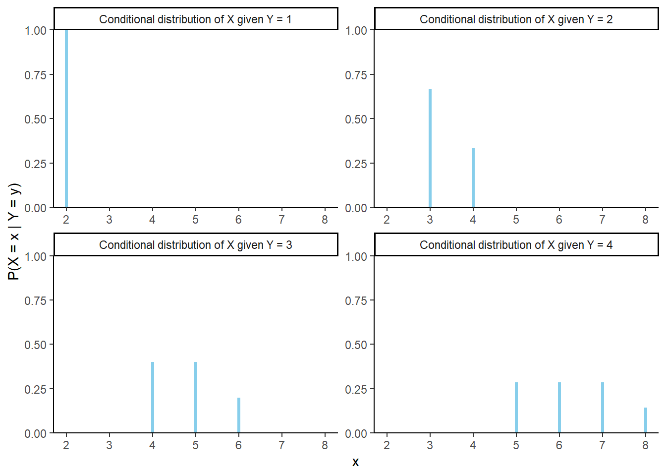
Figure 2.42: Impulse plots representing the family of conditional distributions of $X$ given $Y$. Each plot represents a conditional distribution of $X$ given $Y=y$ for a particular value of $y= 1, 2, 3, 4$.

$Spinners representing the family of conditional distributions of $X$ given $Y$. Each spinner represents a conditional distribution of $X$ given $Y=y$ for a particular value of $y= 1, 2, 3, 4$.$

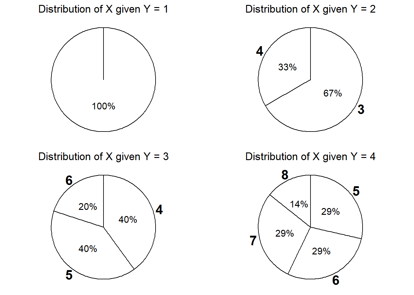
Figure 2.43: Spinners representing the family of conditional distributions of $X$ given $Y$. Each spinner represents a conditional distribution of $X$ given $Y=y$ for a particular value of $y= 1, 2, 3, 4$.

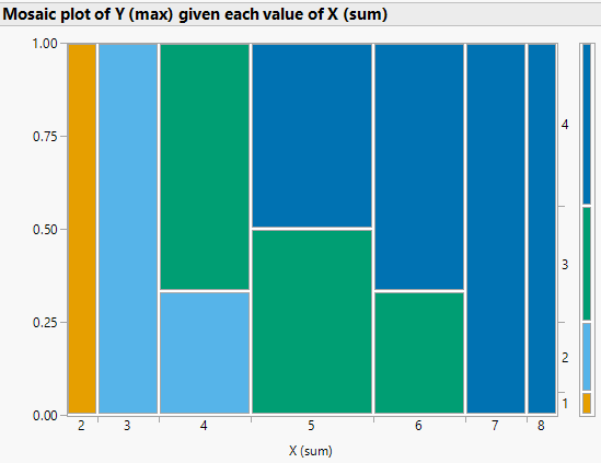
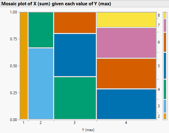
$Mosaic plots for Example 2.59, where $X$ is the sum and $Y$ is the max of two rolls of a fair four-sided die. The plot on the left represents conditioning on values of the sum $X$; color represents values of $Y$. The plot on the right represents conditioning on values of the max $Y$; color represents values of $X$.$ $Mosaic plots for Example 2.59, where $X$ is the sum and $Y$ is the max of two rolls of a fair four-sided die. The plot on the left represents conditioning on values of the sum $X$; color represents values of $Y$. The plot on the right represents conditioning on values of the max $Y$; color represents values of $X$.$

Figure 2.44: Mosaic plots for Example 2.59, where $X$ is the sum and $Y$ is the max of two rolls of a fair four-sided die. The plot on the left represents conditioning on values of the sum $X$; color represents values of $Y$. The plot on the right represents conditioning on values of the max $Y$; color represents values of $X$.

The conditional distribution of $Y$ given $X=x$ is the distribution of $Y$ values over only those outcomes for which $X=x$. It is a distribution on values of $Y$ only; treat $x$ as a fixed constant when conditioning on the event $\{X=x\}$.

Conditional distributions can be obtained from a joint distribution by slicing and renormalizing. The conditional distribution of $Y$ given $X=x$, where $x$ represents a particular number, can be thought of as:

the slice of the joint distribution corresponding to $X=x$, a distribution on values of $Y$ alone with $X=x$ fixed
renormalized so that the slice accounts for 100% of the probability over the values of $Y$

The shape of the conditional distribution of $Y$ given $X=$ is determined by the shape of the slice of the joint distribution over values of $Y$ for the fixed $x$.

For each fixed $x$, the conditional distribution of $Y$ given $X=x$ is a different distribution on values of the random variable $Y$. There is not one “conditional distribution of $Y$ given $X$”, but rather a family of conditional distributions of $Y$ given different values of $X$.

Each conditional distribution is a distribution, so we can summarize its characteristics like mean and standard deviation. The conditional mean and standard deviation of $Y$ given $X=x$ represent, respectively, the long run average and variability of values of $Y$ over only $(X, Y)$ pairs with $X=x$. Since each value of $x$ typically corresponds to a different conditional distribution of $Y$ given $X=x$, the conditional mean and standard deviation will typically be functions of $x$.

Example 2.60 We have already discussed two ways for simulating an $(X, Y)$ pair in the dice rolling example: simulate a pair of rolls and measure $X$ (sum) and $Y$ (max), or spin the joint distribution spinner for $(X, Y)$ once.

Now describe another way for simulating an $(X, Y)$ pair using the spinners in Figure 2.43. (Hint: you’ll need one more spinner in addition to the four from the previous example.)
Describe in detail how you can simulate $(X, Y)$ pairs and use the results to approximate $\textrm{P}(X = 6 | Y = 4)$.
Describe in detail how you can simulate $(X, Y)$ pairs and use the results to approximate the conditional distribution of $X$ given $Y = 4$.
Describe in detail how you can simulate values from the conditional distribution of $X$ given $Y=4$ without simulating $(X, Y)$ pairs.
We have seen that the long run average value of $X$ is 5. Would you expect the conditional long run average value of $X$ given $Y= 4$ to be greater than, less than, or equal to 5? Explain without doing any calculations. What about given $Y = 2$?
How could you use simulation to approximate the conditional long run average value of $X$ given $Y = 4$?

Solution. to Example 2.60

Show/hide solution

Simulate a value of $Y$ from its marginal distribution (e.g., using the spinner in Figure 2.31.) Then given that $y$ is the simulated value of $Y$, simulate a value of $X$ from the conditional distribution of $X$ given $Y=y$ (e.g., using the appropriate spinner from the family of spinners in Figure 2.43). For example, if $Y=4$, simulate a value of $X$ from a distribution that returns the values 5, 6, 7, 8 with probability 2/7, 2/7,2/7, 1/7.
Simulate many $(X, Y)$ pairs (using any appropriate method). Discard any pairs for which $Y\neq 4$. Among the remaining pairs (all with $Y = 4$) count the number of pairs in which $X = 6$, then divide by the total number of pairs with $Y = 4$ to obtain the conditional relative frequency that $X=6$ given $Y=4$. The margin of error is based on the number of simulated repetitions for which $Y=4$.
Continue as in the previous part, but find the conditional relative frequency of each possible $X$ value. We condition on the value of $Y$, but we summarize the simulated $X$ values to approximate the conditional distribution of $X$ given the value of $Y$.
Construct a spinner according to the conditional distribution of $X$ given $Y=4$ (like in Figure 2.43) and spin it. Of course, this requires us to first find the conditional distribution of $X$ given $Y=4$, but in some problems conditional distributions are provided directly.
Unconditionally, $X$ takes values from 2 to 8. Given $Y = 4$, $X$ can only take values 5 to 8. $X$ has a tendency to be larger when $Y=4$ than overall, so we expect the conditional long run average value of $X$ when $Y = 4$ to be greater than 5, the overall average value of $X$. On the other hand, when $Y=2$, $X$ tends to be smaller than overall, so we expect the conditional long run average value of $X$ given $Y=2$ to be less than 5.
Simulate many values of $X$ from the conditional distribution of $X$ given $Y=4$ (using one of the methods described above) and average the simulated values. Notice that we are conditioning on the value of $Y$ but we are averaging the simulated $X$ values.

Rather than directly simulating from a joint distribution, we can simulate an $(X, Y)$ pair in two stages:

Simulate a value of $X$ from its marginal distribution. Call the simulated value $x$.
Given $x$, simulate a value of $Y$ from the conditional distribution of $Y$ given $X = x$. There will be a different distribution (spinner) for each possible value of $x$.

This “marginal then conditional” process is essentially implementing the multiplication rule \[ \text{joint} = \text{conditional}\times\text{marginal} \]

In the dice rolling problem, the “marginal then conditional” method is a lot more trouble than its worth. However, in many problems a joint distribution is described by specifying the marginal distribution of $X$ and the family of conditional distributions of $Y$ given values of $X$, and so the “marginal then conditional” method is the natural way of simulating from a joint distribution.

Recall that we can implement conditioning in Symbulate using |.


P = DiscreteUniform(1, 4) ** 2

X = RV(P, sum)
Y = RV(P, max)

( (X & Y) | (Y == 4) ).sim(10)

Index	Result
0	(6, 4)
1	(6, 4)
2	(8, 4)
3	(7, 4)
4	(7, 4)
5	(8, 4)
6	(7, 4)
7	(7, 4)
8	(8, 4)
...	...
9	(7, 4)


(X | (Y == 4) ).sim(10000).tabulate()

Value	Frequency
5	2879
6	2833
7	2876
8	1412
Total	10000


(X | (Y == 4) ).sim(10000).tabulate(normalize = True)

Value	Relative Frequency
5	0.2873
6	0.2867
7	0.2853
8	0.1407
Total	1.0

Below we simulate from the conditional distribution of $X$ given $Y=y$ for each of the values $y = 2, 3, 4$. Each of the three simulations below approximates a separate conditional distribution of $X$ values.


x_given_Y_eq4 = (X | (Y == 4) ).sim(10000)

x_given_Y_eq3 = (X | (Y == 3) ).sim(10000)

x_given_Y_eq2 = (X | (Y == 2) ).sim(10000)

We plot the three distributions on a single plot to compare how the distribution of $X$ changes depending on the given value of $Y$.

x_given_Y_eq4.plot()
x_given_Y_eq3.plot(jitter = True) # shifts the spikes a little
x_given_Y_eq2.plot(jitter = True) # so they don't overlap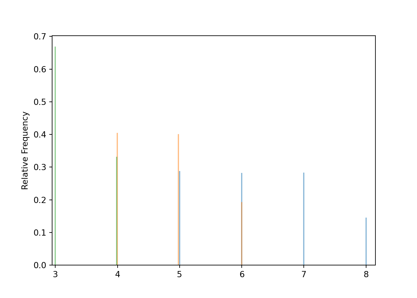

Each conditional distribution is a distribution, so we can summarize its characteristics like mean and standard deviation. Notice how the conditional mean and standard deviation of $X$ depend on the given value of $Y$.

x_given_Y_eq4.mean(), x_given_Y_eq4.sd()

## (6.2874, 1.03585773154425)

x_given_Y_eq3.mean(), x_given_Y_eq3.sd()

## (4.7882, 0.7442719664208776)

x_given_Y_eq2.mean(), x_given_Y_eq2.sd()

## (3.3315, 0.47075232341434065)

2.13.2 Conditional distributions of continuous random variables

For two continuous random variables $X$ and $Y$, the conditional distribution of $Y$ given a particular value $x$ of $X$ can be obtained by from the slice of the joint density surface corresponding to $x$. However, care must be taken when simulating and interpreting conditional distributions given the values of a continuous random variable.

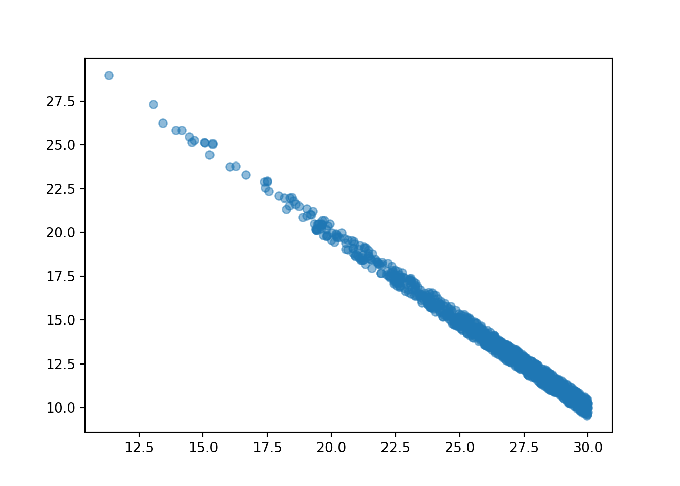
Throughout this section we consider again the case of the meeting problem which assumes that the $(R, Y)$ pairs of arrival times follow a Bivariate Normal distribution with means (30, 30), standard deviations (10, 10) and correlation 0.7. The joint distribution of $R$ and $Y$ is depicted in Figure 2.41.

Example 2.61 Provide answers to the following questions without doing any calculations. It helps to think of the “long run” here as Regina and Cady meeting for lunch each day over many days.

Interpret $\textrm{P}(Y < 30 | R = 40)$ in context. Is $\textrm{P}(Y < 30 | R = 40)$ greater than, less than, or equal to $\textrm{P}(Y < 30)$?
Interpret $\textrm{P}(Y < 30 | R = 15)$ in context. Is $\textrm{P}(Y < 30 | R = 15)$ greater than, less than, or equal to $\textrm{P}(Y < 30)$?
Interpret $\textrm{P}(Y < R | R = 40)$ in context. Is $\textrm{P}(Y < R | R = 40)$ greater than, less than, or equal to $\textrm{P}(Y < R)$?
Interpret the conditional long run average value of $Y$ given $R= 40$ in context. Is it greater than, less than, or equal to 30?
Interpret the conditional long run average value of $Y$ given $R= 15$ in context. Is it greater than, less than, or equal to 30?
Interpret the conditional standard deviation of $Y$ given $R= 40$ in context. Is it greater than, less than, or equal to 10?
Interpret the conditional standard deviation of $Y$ given $R= 15$ in context. Is it greater than, less than, or equal to 10?

Solution. to Example 2.61

Show/hide solution

$\textrm{P}(Y < 30 | R = 40)$ is the conditional probability that Cady arrives before 12:30 given that Regina arrives at 12:40. Among the days on which Regina arrives at 12:40, what proportion of these days does Cady arrive before 12:30? $\textrm{P}(Y < 30 | R = 40)$ is less than $\textrm{P}(Y < 30)=0.5$ since if Regina arrives later (after the mean of 12:30) then Cady tends to arrive later too. So the relative frequency of days on which Cady arrives before 12:30 is less among only days where Regina arrives at 12:40 than among all days. (Look at the slice of the joint distribution corresponding to $R=15$; almost all of the density along this slice lies above $Y < 30$.)
$\textrm{P}(Y < 30 | R = 15)$ is the conditional probability that Cady arrives before 12:30 given that Regina arrives at 12:15. Among the days on which Regina arrives at 12:15, what proportion of these days does Cady arrive before 12:30? $\textrm{P}(Y < 30 | R = 15)$ is greater than $\textrm{P}(Y < 30) = 0.5$ since if Regina arrives earlier (before the mean of 12:30) then Cady tends to arrive earlier too. So the relative frequency of days on which Cady arrives before 12:30 is greater among only days where Regina arrives at 12:15 than among all days. (Look at the slice of the joint distribution corresponding to $R=15$; almost all of the density along this slice lies below $Y < 30$.)
$\textrm{P}(Y < R | R = 40)$ is the conditional probability that Cady arrives before Regina given that Regina arrives at 12:40. Among the days on which Regina arrives at 12:40, what proportion of these days is Cady the first to arrive? $\textrm{P}(Y < R | R = 40)$ is greater than $\textrm{P}(Y < R) = 0.5$ since if Regina arrives later (after the mean of 12:30) then Cady has “more room” to arrive early. (Look at the slice of the joint distribution corresponding to $R=40$; a larger portion of the density along this slice lies below $Y = 40$ than above.) So the relative frequency of days on which Cady arrives before Regina is greater among only days where Regina arrives at 12:40 than among all days.
$\textrm{P}(Y < R | R = 15)$ is the conditional probability that Cady arrives before Regina given that Regina arrives at 12:15. Among the days on which Regina arrives at 12:15, what proportion of these days is Cady the first to arrive? $\textrm{P}(Y < R | R = 15)$ is less than $\textrm{P}(Y < R) = 0.5$ since if Regina arrives earlier (before the mean of 12:30) then Cady has “less room” to arrive early. (Look at the slice of the joint distribution corresponding to $R=15$; a larger portion of the density along this slice lies above $Y = 15$ than below.) So the relative frequency of days on which Cady arrives before Regina is smaller among only days where Regina arrives at 12:15 than among all days.
The conditional long run average value of $Y$ given $R= 40$ is the average of Cady’s arrival times on days where Regina arrives at 12:40. It is greater than 30 — Cady’s average arrival time overall days — since if Regina arrives later (after the mean of 30) then Cady also tends to arrive later.
The conditional long run average value of $Y$ given $R= 15$ is the average of Cady’s arrival times on days where Regina arrives at 12:15. It is less than 30 — Cady’s average arrival time overall all days — since if Regina arrives earlier (before the mean of 30) then Cady also tends to arrive earlier.
The conditional standard deviation of $Y$ given $R= 40$ measures the variability of Cady’s arrival times on days where Regina arrives at 12:40. It is less than 10 — the overall variability of Cady’s arrival times — since days on which Regina arrives at 12:40 form a more homogeneous group of days. Compare the overall range of $Y$ values with the range of $Y$ values which accounts for almost all of the density along the $R=40$ slice of the joint distribution.
The conditional standard deviation of $Y$ given $R= 15$ measures the variability of Cady’s arrival times on days where Regina arrives at 12:15. It is less than 10 — the overall variability of Cady’s arrival times — since days on which Regina arrives at 12:15 form a more homogeneous group of days. Compare the overall range of $Y$ values with the range of $Y$ values which account for almost all of the density along the $R=15$ slice of the joint distribution.

We repeat here some of the ideas we introduced for discrete random variables. The concepts are analogous for continuous random variables. The main difference is that continuous random variables are represented by density curves (or surfaces) where areas (or volumes) determine probabilities.

the slice of the joint distribution corresponding to $X=x$, a distribution on values of $Y$ alone with $X=x$ fixed
renormalized so that the slice accounts for 100% of the probability over the values of $Y$. The slice now represents the distribution of a single continuous random variable $Y$. Remember that the distribution of a continuous random variable is represented by a density where area determines probability.

The shape of the conditional distribution of $Y$ given $X=$ is determined by the shape of the slice of the joint distribution over values of $Y$ for the fixed $x$.

The plot below depicts the joint distribution of $R$ and $Y$ with the slices for $R = 40$ (orange) and $R=15$ (purple) highlighted.

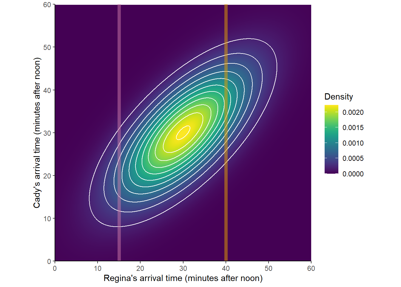
Figure 2.45: A Bivariate Normal distribution with two slices highlighted

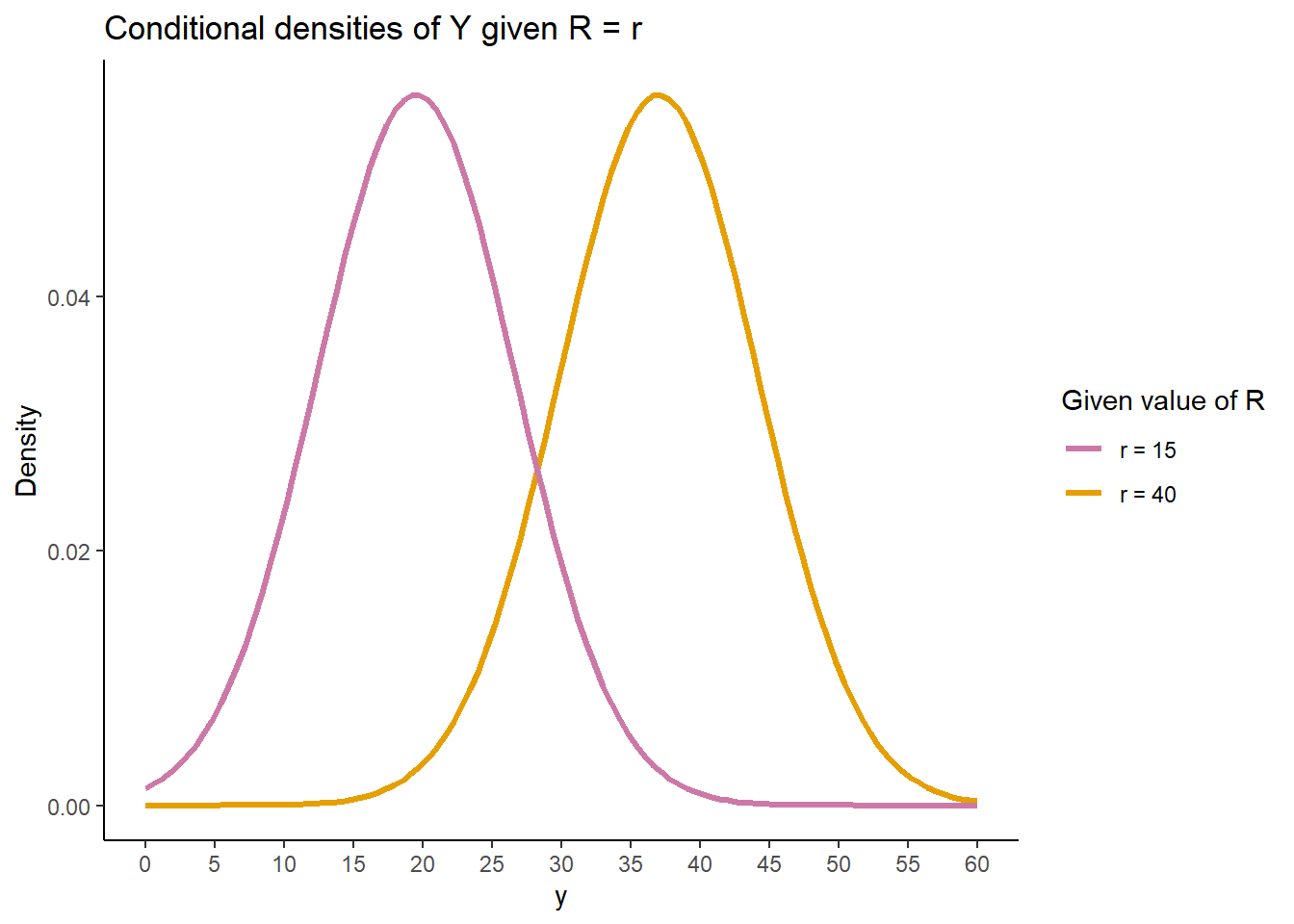
The slices in the previous plot determine the shapes of the conditional distributions of $Y$ given $R=40$ and given $R=15$. In the joint distribution, each of the slices corresponds to a certain area. Now for each slice we rescale the density so that the rescaled area represents 100% of the probability. The plot below depicts the two conditional distributions. Pay attention to the horizonal axis! These are distributions over values of $Y$; values of $Y$ are represented on the horizontal axis below.

It is hard to visualize the exact shape of the slices in the joint distribution. However, from the joint distribution picture we can get an idea of how the conditional mean of $Y$ changes with the values of $R$, and that the conditional standard deviation of $Y$ given any particular value of $R$ is less than the overall standard deviation of $Y$. From the density color along a vertical slice, we see that density tends to be highest around the mean for the slice (conditional mean of $Y$ given $R=r$) and then decreases relatively symmetrically, suggest at least a symmetric conditional density. (If turns out that is $X$ and $Y$ have a Bivariate Normal distribution, then the conditional distribution of $Y$ given $X=x$ is Normal, for any $x$.)

Many concepts are analogous for discrete and continuous random variables. However, extra care is required when simulating and interpreting conditional distributions given the values of a continuous random variable.

Example 2.62 Donny Don’t writes the following Symbulate code to approximate the conditional distribution of $Y$ given $R=40$, the conditional distribution of Cady’s arrival time given Regina arrives at 12:40. What do you think will happen when Donny runs his code?

R, Y = RV(BivariateNormal(mean1 = 30, sd1 = 10, mean2 = 30, sd2 = 10, corr = 0.7))

(Y | (R == 40) ).sim(10000)

Solution. to Example 2.62

Show/hide solution

Donny’s code will run forever! Remember, $R$ is a continuous random variable, so $\textrm{P}(R = 40)=\textrm{P}(R = 40.00000000000000000\ldots) = 0$. The simulation will never return a single value of $(R, Y)$ with $Y$ equal to $40.0000000000000\ldots$, let alone 10000 of them.

Be careful when conditioning with continuous random variables. Remember that the probability that a continuous random variable is equal to a particular value is 0; that is, for continuous $X$, $\textrm{P}(X=x)=0$. Mathematically, when we condition on $\{X=x\}$ we are really conditioning on $\{|X-x|<\epsilon\}$ — the event that the random variable $X$ is within $\epsilon$ of the value $x$ — and seeing what happens in the idealized limit when $\epsilon\to0$. Practically, $\epsilon$ represents our “close enough” degree of precision, e.g., $\epsilon=0.01$ if “within 0.01” is close enough. In the meeting problem, when we say “Regina arrives at 12:40”, we really mean something like “Regina arrives within one minute of 12:40”. When conditioning on a continuous random variable $X$ in a simulation, never condition on $\{X=x\}$; rather, condition on $\{|X-x|<\epsilon\}$ where $\epsilon$ represents the suitable degree of precision.

To avoid conditioning on the event $\{X = x\}$, which has 0 probability, we need to condition on an event like $\{|X-x|<\epsilon\}$ which often has low probability. Conditioning on low probability events introduces some computational challenges. Remember that the margin of error in using a relative frequency to approximate a probability is based on the number of independently simulated repetitions used to compute the relative frequency. When approximating a conditional probability with a conditional relative frequency, the margin of error is based only on the number of repetitions that satisfy the condition. (Likewise for using simulated averages to approximate long run averages.) Naively discarding repetitions that do not satisfy the condition can be horribly inefficient. For example, when conditioning on an event with probability 0.01 we would need to run about 1,000,000 repetition to achieve 10,000 that satisfy the condition. There are more sophisticated and efficient methods (e.g. “Markov chain Monte Carlo (MCMC)” methods), but they are beyond the scope of this book. When conditioning on the value of a continuous random variable with | in Symbulate, be aware that you might need to change either the number of repetitions (but try not to go below 1000) or the degree of precision $\epsilon$.

The code below approximates conditioning on the event $\{R = 40\}$ by conditioning instead on the event that $R$ rounded to the nearest minute is 40 , $\{|R - 40| < 0.5\} = \{39.5<R<40.5\}$, an event which has probability 0.04 (since $R$ has a Normal(30, 10) distribution.)


R, Y = RV(BivariateNormal(mean1 = 30, sd1 = 10, mean2 = 30, sd2 = 10, corr = 0.7))

( (R & Y) | (abs(R - 40) < 0.5) ).sim(10)

Index	Result
0	(39.537474809255656, 36.126472896647215)
1	(40.266040494221244, 48.02348200199232)
2	(40.40399994166887, 42.07538524670129)
3	(39.72373534162258, 44.98036662147892)
4	(39.68126886096103, 43.10380822274939)
5	(39.874751168850075, 39.467175208375025)
6	(40.13532828513675, 38.520947436639574)
7	(39.67168173710453, 43.53578352384494)
8	(39.97316309256614, 39.983793282217135)
...	...
9	(40.38138767037978, 28.607343540589508)

Now we approximate the conditional distribution of $Y$ given $R=40$ and some of its features. Running (Y | (abs(R - 40) < 0.5) ).sim(1000) requires about 25000 repetitions in the background to achieve the 1000 the satisfy the condition. The margin of error for approximating conditional probabilities is roughly $1/\sqrt{1000} = 0.03$.


y_given_R_eq40 = ( Y | (abs(R - 40) < 0.5) ).sim(1000)

The above simulates many $Y$ values given the condition. We can visualize the simulated values in a histogram; compare to the orange density in ??.

y_given_R_eq40.plot()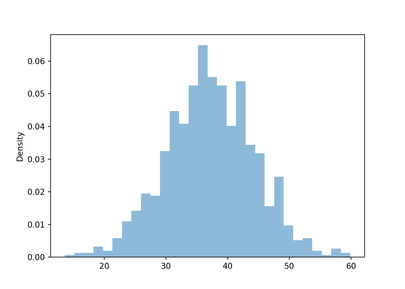

Now we approximate some features of the conditional distribution relating to Example 2.61. For example, the simulation suggests that $\textrm{P}(Y < 30 | R = 40)$ is less than $\textrm{P}(Y < 30) = 0.5$. (But keep in mind that the simulated relative frequencies are really $\pm 0.03$.) Compare the simulated values below to our responses to Example 2.61.

Approximate $\textrm{P}(Y < 30 | R = 40)$ is less than $\textrm{P}(Y < 30) = 0.5$:

y_given_R_eq40.count_lt(30) / y_given_R_eq40.count()

## 0.154

Approximate $\textrm{P}(Y < R | R = 40)$ is greater than $\textrm{P}(Y < R) = 0.5$:

y_given_R_eq40.count_lt(40) / y_given_R_eq40.count()

## 0.656

Approximate long run average of $Y$ given $R = 40$ is greater than 30 (overall average value of $Y$):

y_given_R_eq40.mean()

## 37.15746879025182

Approximate standard deviation of $Y$ given $R = 40$ is less than 10 (overall standard deviation of $Y$):

y_given_R_eq40.sd()

## 7.1428141789224995

Now we condition on $R= 15$ and compare. (We’re conditioning on an even lower probability event now.)


y_given_R_eq15 = ( Y | (abs(R - 15) < 0.5) ).sim(1000)

We can visualize the simulated values in a histogram; compare to the densities in ??. We see that the conditional distribution of $Y$ given $R=r$ changes based on the value of $r$.

y_given_R_eq40.plot()
y_given_R_eq15.plot()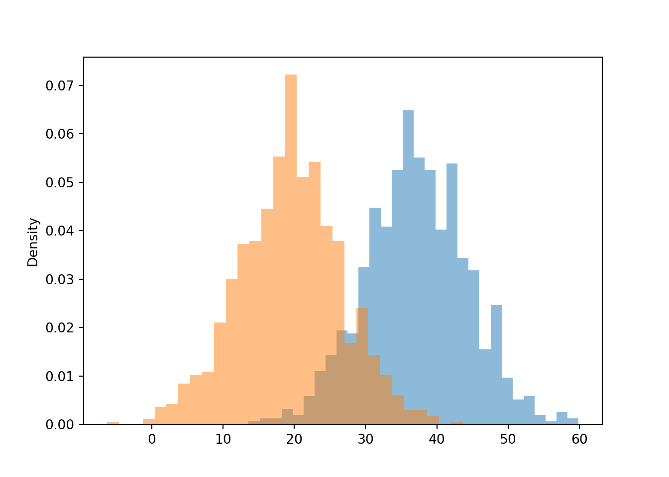

Approximate $\textrm{P}(Y < 30 | R = 15)$ is greater than $\textrm{P}(Y < 30) = 0.5$:

y_given_R_eq15.count_lt(30) / y_given_R_eq15.count()

## 0.927

Approximate $\textrm{P}(Y < R | R = 15)$ is less than $\textrm{P}(Y < R) = 0.5$:

y_given_R_eq15.count_lt(15) / y_given_R_eq15.count()

## 0.254

Approximate long run average of $Y$ given $R = 15$ is less than 30 (overall average value of $Y$):

y_given_R_eq15.mean()

## 19.466111145624716

Approximate standard deviation of $Y$ given $R = 15$ is less than 10 (overall standard deviation of $Y$):

y_given_R_eq15.sd()

## 7.1254517676259

In some problems, the joint distribution is naturally specified by describing the marginal distribution of one of the variables, and the family of conditional distributions of the other variable given values of the first.

Example 2.63 In the meeting problem, assume that $R$ follows a Normal(30, 10) distribution. For any value $r$, assume that the conditional distribution of $Y$ given $R=r$ is a Normal distribution with mean $30 + 0.7(r - 30)$ and standard deviation 7.14 minutes.

How can we simulate a value of $R$ using only the standard Normal spinner from Figure 2.38?
Suppose the simulated value of $R$ is 40. What is the distribution that we want to simulate the corresponding $Y$ value from?
How can we simulate a value of $Y$ from the distribution in the previous part using only the standard Normal spinner?
Now suppose the simulated value of $R$ is 15. What is the distribution that we want to simulate the corresponding $Y$ value from?
How can we simulate a value of $Y$ from the distribution in the previous part using only the standard Normal spinner?
Suggest a general method for simulating an $(R, Y)$ pair.
Simulate many $(R, Y)$ pairs and summarize the results, including the correlation. (See code below.) How does the simulated joint distribution compare to the Bivariate Normal distribution from Example 2.61?
What is the approximate marginal distribution of $Y$?

Solution. to Example 2.63

The standard Normal spinner simulates standardized values. For example, if the spinner returns a value of 1, that means 1 standard deviation above the mean, or $30+(1)10=40$ in the meeting problem. Spin the standard Normal spinner once and let the result be $Z_1$, then set $R = 30 + 10Z_1$. Then the simulated $R$ values will follow a Normal(30, 10) distribution.
The assumed conditional distribution of $Y$ given $R=40$ is Normal with mean $30 + 0.7(40 - 30) = 37$ and standard deviation 7.14 minutes. So if $R=40$ we want to simulate $Y$ from a Normal(37, 7.14) distribution.
Spin the standard Normal spinner again, call the result $Z_2$, and set $Y= 37 + 7.14Z_2$. $Y$ values simulated in this way will follow a Normal(37, 7.14) distribution.
The assumed conditional distribution of $Y$ given $R=15$ is Normal with mean $30 + 0.7(15 - 30) = 19.5$ and standard deviation 7.14 minutes. So if $R=15$ we want to simulate a value from a Normal(19.5, 7.14) distribution.
Spin the standard Normal spinner again, call the result $Z_2$, and set $Y= 19.5 + 7.14Z_2$. $Y$ values simulated in this way will follow a Normal(19.5, 7.14) distribution.
Spin the standard Normal spinner twice, and call the results $Z_1, Z_2$. Set $R = 30 + 10Z_1$. Whatever $R$ is, we want the corresponding conditional mean of $Y$ to be $30 + 0.7(R - 30)$, so set $Y = 30 + 0.7(R - 30) + 7.14Z_2$.
See the results below. The correlation is about 0.7 and the joint distribution of $R$ and $Y$ looks pretty similar to the Bivariate Normal distribution we had assumed previously.
See the simulation results below. The marginal distribution of $Y$ is approximately Normal(30, 10).

Z1, Z2 = RV(Normal(0, 1) ** 2)

R = 30 + 10 * Z1

Y = 30 + 0.7 * (R - 30) + 7.14 * Z2

r_and_y = (R & Y).sim(10000)

r_and_y.corr()

## 0.7023093876861758

The correlation is approximately 0.7. The marginal means are both approximately 30.

r_and_y.mean()

## (30.179067810894672, 30.14122543070981)

And the marginal standard deviations are both approximately 10.

r_and_y.sd()

## (10.08426841220993, 10.035469259222562)

Plots of simulated values look similar to the Bivariate Normal distribution case.

r_and_y.plot()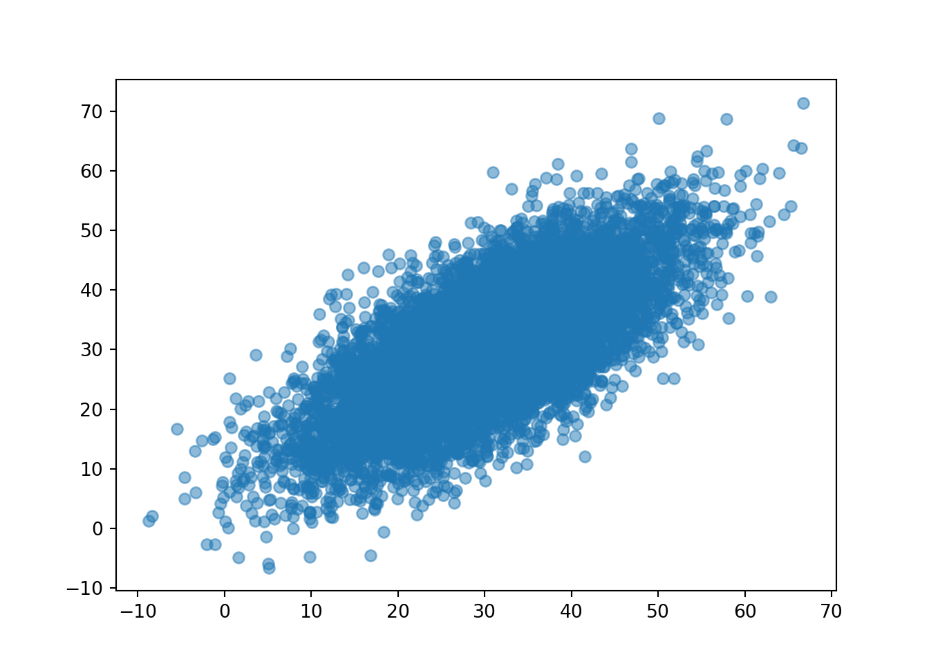

r_and_y.plot('hist')

## Error in py_call_impl(callable, dots$args, dots$keywords): ValueError: invalid literal for int() with base 10: ''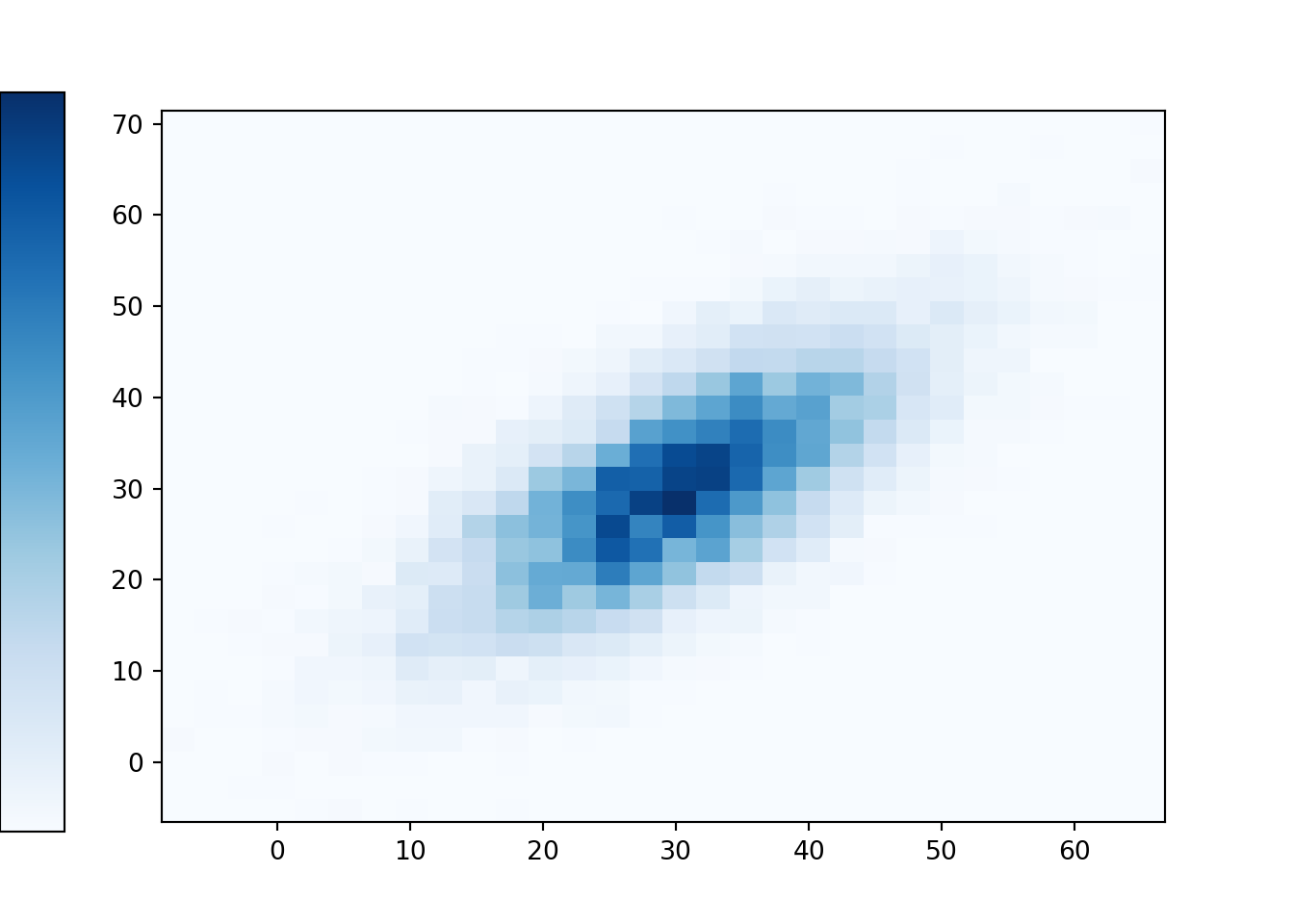

The marginal distribution of $Y$ is approximately Normal with mean 30 and standard deviation 10. Notice that while the conditional mean of $Y$ changes with $R$, the overall marginal mean of $Y$ is 30. Also, while the variability of $Y$ for any given value of $R$ is 7.14, the overall variability of $Y$ is 10.

y = r_and_y[1]

y.mean(), y.sd()

## (30.141225430709753, 10.03546925922256)

y.plot()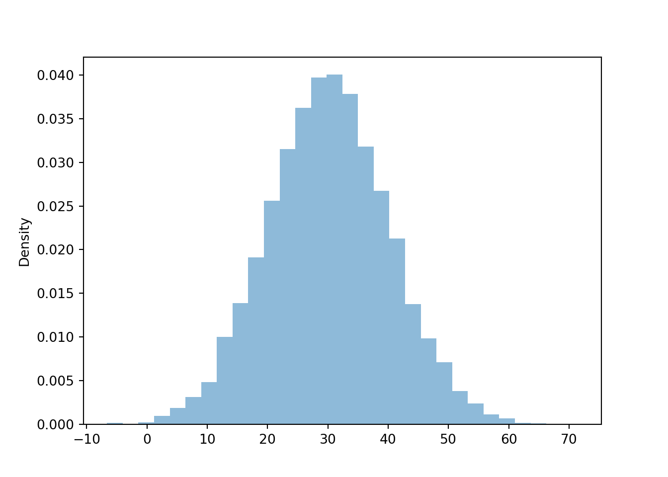

The above example provides one method for simulating from a Bivariate Normal distribution using only a standard Normal spinner. We willl study Bivariate Normal distributions in more detail later.

Be sure to distinguish between joint, conditional, and marginal distributions.

The joint distribution is a distribution on $(X, Y)$ pairs. A mathematical expression of a joint distribution is a function of both values of $X$ and values of $Y$.
The conditional distribution of $Y$ given $X=x$ is a distribution on $Y$ values (among $(X, Y)$ pairs with a fixed value of $X=x$). A mathematical expression of a conditional distribution will involve both $x$ and $y$, but $x$ is treated like a fixed constant and $y$ is treated as the variable. Note: the possible values of $Y$ might depend on the value of $x$.
The marginal distribution of $Y$ is a distribution on $Y$ values only, regardless of the value of $X$. A mathematical expression of a marginal distribution will have only values of the single variable in it; for example, an expression for the marginal distribution of $Y$ will only have $y$ in it (no $x$, not even in the possible values).

We have focused on the conditional distribution of one random variable $Y$ given the value $x$ of another random variable $X$. But we can also consider how joint distributions change with conditioning. For example, the following simulates values of $T$ and $W$ (first time, waiting time) in the meeting problem given $R= 40$.

W = abs(R - Y)

T = (R & Y).apply(min)

t_and_w_given_R_eq40 = ( (T & W) | (abs(R - 40) < 0.5) ).sim(1000)

t_and_w_given_R_eq40.corr()

## -0.8034692480153036

t_and_w_given_R_eq40.plot()

We can also condition on events other than “equals to” events, and events involving multiple random variables. Below we simulate the joint distribution of $T$ and $W$ given $R = 40$ and $Y < 30$. (Note that & plays a different role on either side of the conditioning |.)

W = abs(R - Y)

T = (R & Y).apply(min)

t_and_w_given_R_eq40_and_Y_lt30 = ( (T & W) | ( (abs(R - 40) < 0.5) & (Y < 30) ) ).sim(1000)

t_and_w_given_R_eq40_and_Y_lt30.corr()

## -0.9960667035189514

t_and_w_given_R_eq40_and_Y_lt30.plot()