7.1 Exponential distributions

Exponential distributions are often used to model the waiting times between events in a random process that occurs continuously over time.

Example 7.1 Suppose that we model the time, measured continuously in hours, from now until the next earthquake (of any magnitude) occurs in southern CA as a continuous random variable $X$ with pdf \[ f_X(x) = 2 e^{-2x}, \; x \ge0 \]

Sketch the pdf of $X$. What does this tell you about waiting times?
Without doing any integration, approximate the probability that $X$ rounded to the nearest minute is 0.5 hours.
Compute and interpret $\textrm{P}(X \le 3)$.
Find the cdf of $X$.
Find the median time between earthquakes.
Set up the integral you would solve to find $\textrm{E}(X)$. Interpret $\textrm{E}(X)=1/2$. How does the median compare to the mean? Why?
Set up the integral¹³⁵ you would solve to find $\textrm{E}(X^2)$.
Find $\textrm{Var}(X)$ and $\textrm{SD}(X)$.

Solution. to Example 7.1

Show/hide solution

See simulation below for plots. Waiting times near 0 are most likely, and density decreases as waiting time increases.
Remember, the density at $x=0.5$ is not a probability, but it is related to the probability that $X$ takes a value close to $x=0.5$. The approximate probability that $X$ rounded to the nearest minute is 0.5 hours is \[ f_X(0.5)(1/60) = 2e^{-2(0.5)}(1/60) = 0.0123 \]
$\textrm{P}(X \le 3) = \int_0^3 2e^{-2x}dx = 1-e^{-2(3)}=0.9975$. While any value greater than 0 is possible in principle, the probability that $X$ takes a really large value is small. About 99.75% of earthquakes happen within 3 hours of the previous earthquake.
$F_X(x)=0$ for $x<0$. For $x>0$, repeat the calculation from the previous part with a generic $x>0$. \[ F_X(x) =\textrm{P}(X \le x) = \int_0^x 2e^{-2u}du = 1-e^{-2x} \]
Set $0.5=F_X(m)=1-e^{-2m}$ and solve for $m=(1/2)\log(2) = 0.347$. About 50% of earthquakes occur within 0.347 hours (about 21 minutes) of the previous earthquake.
$\textrm{E}(X)=\int_0^\infty x \left(2 e^{-2x}\right)dx = 1/2$. The long run average waiting time between earthquakes is 0.5 hours. The mean is greater than the median due to the right tail of the distribution; the extreme large values pull the mean up.
Use LOTUS: $\textrm{E}(X^2)=\int_0^\infty x^2 \left(2 e^{-2x}\right)dx = 1/2$.
$\textrm{Var}(X)=\textrm{E}(X^2) - (\textrm{E}(X))^2=1/2-(1/2)^2=1/4$ and $\textrm{SD}(X)=1/2$.


X = RV(Exponential(rate = 2))

x = X.sim(10000)

x.plot()

Exponential(rate = 2).plot()
plt.show()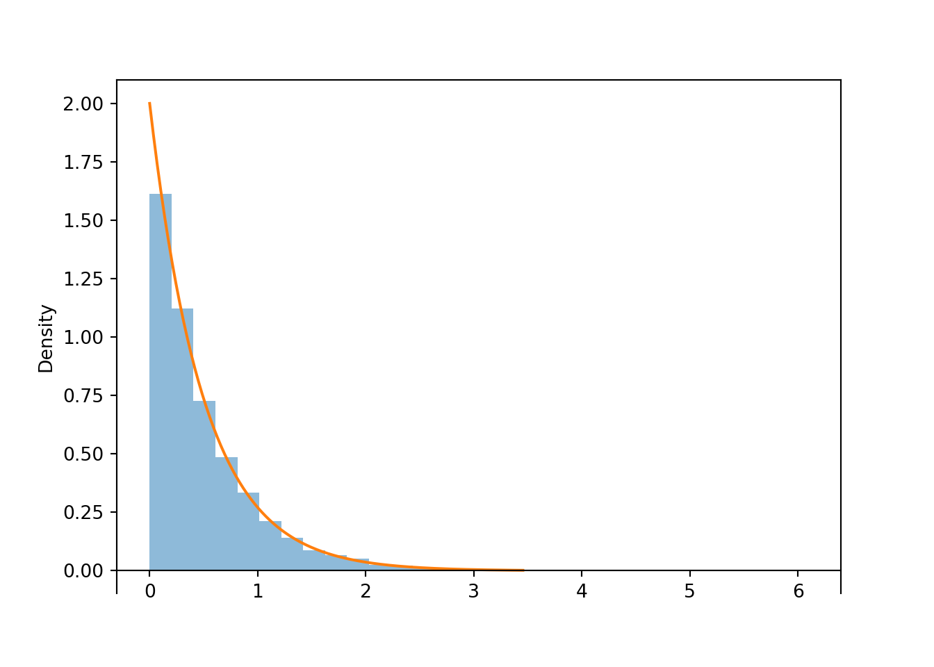


x.count_leq(3) / 10000, Exponential(rate = 2).cdf(3)

## (0.9975, 0.9975212478233336)


x.quantile(0.5), Exponential(rate = 2).quantile(0.5)

## (0.35217190427084516, 0.34657359027997264)


x.mean(), Exponential(rate = 2).mean()

## (0.5042821164386487, 0.5)


x.var(), Exponential(rate = 2).var()

## (0.2563290787926746, 0.25)

Definition 7.1 A continuous random variable $X$ has an Exponential distribution with rate parameter¹³⁶ $\lambda>0$ if its pdf is \[ f_X(x) = \begin{cases}\lambda e^{-\lambda x}, & x \ge 0,\\ 0, & \text{otherwise} \end{cases} \] If $X$ has an Exponential($\lambda$) distribution then \[\begin{align*} \text{cdf:} \quad F_X(x) & = 1-e^{-\lambda x}, \quad x\ge 0\\ \textrm{P}(X>x) & = e^{-\lambda x}, \quad x\ge 0\\ \textrm{E}(X) & = \frac{1}{\lambda}\\ \textrm{Var}(X) & = \frac{1}{\lambda^2}\\ \textrm{SD}(X) & = \frac{1}{\lambda} \end{align*}\]

Exponential distributions are often used to model the waiting time in a random process until some event occurs.

$\lambda$ is the average rate at which events occur over time (e.g., 2 per hour)
$1/\lambda$ is the mean time between events (e.g., 1/2 hour)

plt.figure()
rates = [0.5, 1, 2]
for rate in rates:
    Exponential(rate).plot()
    
plt.legend(['$\lambda=$' + str(i) for i in rates]);
plt.xlim(0, 8);
plt.show()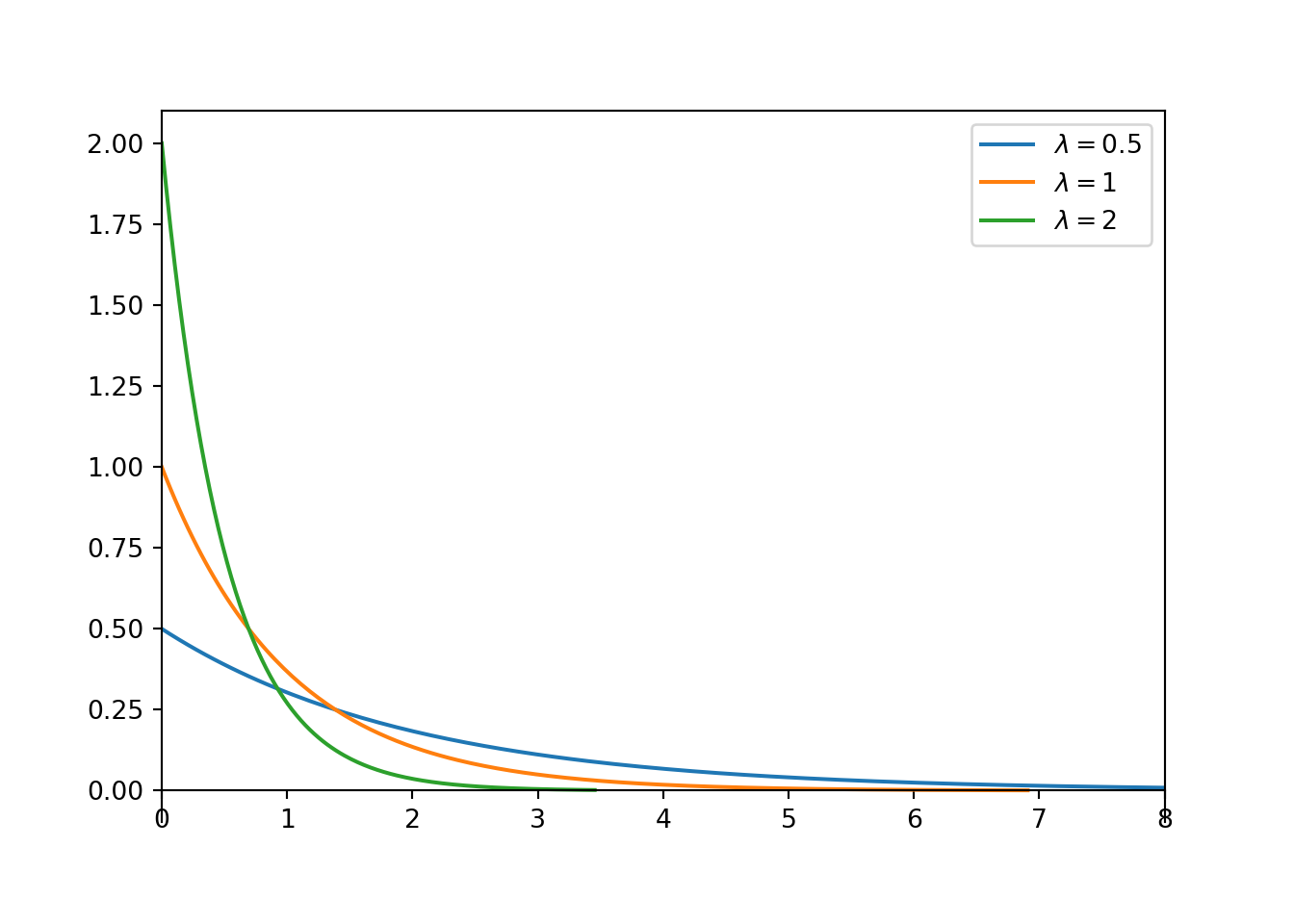

$Exponential densities with rate parameter $\lambda$.$

Figure 7.1: Exponential densities with rate parameter $\lambda$.

Example 7.2 Continuing Example 7.1. Let $Y$ be the time between earthquakes, measured in minutes. Identify the distribution of $Y$ and its mean and standard deviation.

Solution. to Example 7.2

Show/hide solution

If $X$ is waiting time measured in hours, then $Y=60X$ is waiting time measured in minutes. This linear rescaling will not change the shape of the distribution, so $Y$ has an Exponential distribution. If the mean waiting time is $\textrm{E}(X)=1/2$ hours, then $\textrm{E}(Y) = 60(1/2) = 30$ minutes. Likewise, $\textrm{SD}(X) = 1/2$ hour and $\textrm{SD}(Y) = 30$ minutes. Therefore, $Y=60X$ has an Exponential distribution with rate parameter $2/60 = 1/30$ earthquakes per minute.

If $X$ has an Exponential($\lambda)$ distribution and $a>0$ is a constant, then $aX$ has an Exponential($\lambda/a$) distribution.

If $X$ is measured in hours with rate $\lambda = 2$ per hour and mean 1/2 hour
Then $60X$ is measured in minutes with rate $2/60$ per minute and mean $60(1/2)=30$ minutes.

Example 7.3 How do you simulate values from an Exponential distribution?

How could you use an Exponential(1) spinner to simulate values from an Exponential($\lambda$) distribution?
How could you use an Uniform(0, 1) spinner to simulate values from an Exponential($\lambda$) distribution?

Solution. to Example 7.3

Show/hide solution

Spin the Exponential(1) spinner to generate $W$ and the divide $W$ by $\lambda$. If $W$ has an Exponential(1) distribution, then $W/\lambda$ has an Exponential distribution with rate parameter $\lambda$ (and mean $1/\lambda$).
Spin the Uniform(0, 1) spinner to generate $U$ and let $W = -\log(U)$; then $W$ has an Exponential(1) distribution, so $-\log(U)/\lambda$ has an Exponential($\lambda$) distribution.

If $X$ has an Exponential(1) distribution and $\lambda>0$ is a constant then $X/\lambda$ has an Exponential($\lambda$) distribution.

Remember that if $U$ has a Uniform(0, 1) distribution then $-\log(U)$ has Exponential(1) distribution. (Remember also that $-\log(1-U)$ has an Exponential(1) distribution.)

Example 7.4 $X$ and $Y$ are continuous random variables with joint pdf \[ f_{X, Y}(x, y) = \frac{1}{3x^2}\exp\left(-\left(\frac{y}{x^2} + \frac{x}{3}\right)\right), \qquad x > 0, y>0 \]

Identify by name the marginal distribution and one-way conditional distributions that you can obtain from the joint pdf without doing any calculus.
How could you use an an Exponential(1) spinner to simulate $(X, Y)$ pairs with this joint distribution?
Sketch a plot of the joint pdf.
Find $\textrm{E}(Y)$ without doing any calculus.
Find $\textrm{Cov}(X, Y)$ without doing any calculus. (Well, without doing any multivariable calculus.)
Use simulation to approximate the distribution of $Y$. Does $Y$ have an Exponential distribution?

Solution. to Example 7.4

Show/hide solution

Remember that “joint is the product of conditional times marginal”. We can write \[ f_{X, Y}(x, y) = \frac{1}{3x^2}\exp\left(-\frac{y}{x^2}\right) \exp\left(-\frac{x}{3}\right), \qquad x > 0, y>0 \] We can find the conditional pdfs by fixing either variable. Since $x$ shows up in more places, fix $x$ and treat it like a constant and see how the joint pdf depends on $y$. For fixed $x>0$ \[ f_{Y|X}(y|x) \propto \exp\left(-\frac{y}{x^2}\right), \qquad y >0 \] The above has the basic shape of an Exponential pdf with ($1/x^2$) playing the role of the rate parameter. We add the constant in so that it integrates to 1: \[ f_{Y|X}(y|x) = \frac{1}{x^2} \exp\left(-\frac{y}{x^2}\right), \qquad y >0 \] Therefore, for any $x>0$, the conditional distribution of $Y$ given $X=x$ is the Exponential distribution with rate parameter $1/x^2$. Then “joint is the product of conditional times marginal” implies that the marginal pdf of $X$ is \[ f_{X}(x) = \frac{1}{3}\exp\left(-\frac{x}{3}\right), \qquad x > 0 \] Therefore, the marginal distribution of $X$ is the Exponential distribution with rate parameter 1/3.
Spin the Exponential(1) spinner twice and let the results be $U_1, U_2$. Let $X = 3 U_1$. (Remember, if the rate parameter of $X$ is 1/3 then its mean is 3.) Let $Y = X^2 U_2$.
See the simulation results below (and the video). There is a not small probability of some extreme outliers which can obscure the scale on the plot.
Since the conditional distribution of $Y$ given $X=x$ is Exponential with rate parameter $1/x^2$ and mean $x^2$, $\textrm{E}(Y|X) = X^2$. Use the law of total expected value. \[ \textrm{E}(Y) = \textrm{E}(\textrm{E}(Y|X)) = \textrm{E}(X^2) = \textrm{Var}(X) + (\textrm{E}(X))^2 = (3^2) + (3)^2 = 18 \]
$\textrm{Cov}(X, Y) = E(XY) - \textrm{E}(X)\textrm{E}(Y)$. $\textrm{E}(X) = 3$ and $\textrm{E}(Y) = 18$, so we need to find $\textrm{E}(XY)$. Use the law of total expected value and taking out what is known. \[ \textrm{E}(XY) = \textrm{E}(\textrm{E}(XY|X)) = \textrm{E}(X\textrm{E}(Y|X)) = \textrm{E}(X(X^2)) = \textrm{E}(X^3) = \int_0^\infty x^3 \left(\frac{1}{3}e^{-(1/3)x}\right)dx = 162 \] The last integral is a LOTUS calculation. But note that we have reduced $\textrm{E}(XY)$ which on the surface involves a double integral over the joint distribution of $X$ and $Y$ to $\textrm{E}(X^3)$, a calculation which just involves the marginal distribution of $X$. $\textrm{Cov}(X, Y) = 162 - (3)(18)=108$.
See simulation results below. Even though for any value $x$ of $X$ the conditional distribution of $Y$ given $X=x$ is an Exponential distribution, the marginal distribution of $Y$ is not an Exponential distribution. $Y$ has a much heavier tail than an Exponential distribution, and allows for more extreme values than an Exponential distribution does.


U1, U2 = RV(Exponential(1) ** 2)

X = 3 * U1
Y = X ** 2 * U2

(X & Y).sim(100).plot()
plt.show()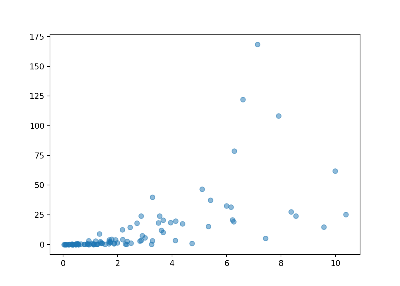


(X & Y).sim(10000).cov()

## 113.44229298529193


y = Y.sim(10000)

y.plot()
plt.show()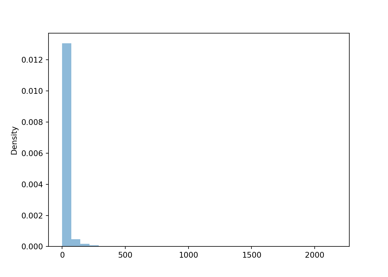


y.mean(), y.sd()

## (18.076512254235137, 57.55534541158378)

7.1.1 Memoryless property

Example 7.5 Let $X$ be the waiting time (hours) until the next earthquake and assume $X$ has an Exponential(2) distribution.

Find the probability that the waiting time is greater than 1 hour.
Suppose that no earthquakes occur in the next 3 hours. Find the conditional probability that the waiting time (from now) is greater than 4 hours. Be sure to write a valid probability statement involving $X$ before computing. What do you notice?

Solution. to Example 7.5

Show/hide solution

$\textrm{P}(X > 1) =e^{-2(1)}$
The event that no earthquakes occur in the next 3 hours is $\{X>3\}$. The conditional probability is \[\begin{align*} \textrm{P}(X > 4 | X > 3) & = \frac{\textrm{P}(X > 4, X>3)}{\textrm{P}(X>3)} \\ & = \frac{\textrm{P}(X > 4)}{\textrm{P}(X>3)}\\ & = \frac{e^{-2(4)}}{e^{-2(3)}}\\ & = e^{-2(1)}\\ & = \textrm{P}(X > 1) \end{align*}\] The conditional probability that we wait for at least one more hour given that we have waited 3 hours already is equal to the unconditional probability that we wait for at least one hour.

Memoryless property. If $W$ has an Exponential($\lambda$) distribution then for any $w,h>0$ \[ \textrm{P}(W>w+h\,\vert\, W>w) = \textrm{P}(W>h) \]

Given that we have already waited $w$ units of time, the conditional probability that we wait at least an additional $h$ units of time is the same as the unconditional probability that we wait at least $h$ units of time.

Probabilistically, the process “forgets” how long we have already waited.

A continuous random variable $W$ has the memoryless property if and only if $W$ has an Exponential distribution. That is, Exponential distributions are the only continuous¹³⁷ distributions with the memoryless property.

If $W$ has an Exponential($\lambda$) distribution then the conditional distribution of the excess waiting time, $W - w$, given $\{W>w\}$ is Exponential($\lambda$).


X = RV(Exponential(rate = 2))

( (X - 3) | (X > 3) ).sim(1000).plot()
Exponential(rate = 2).plot()
plt.show()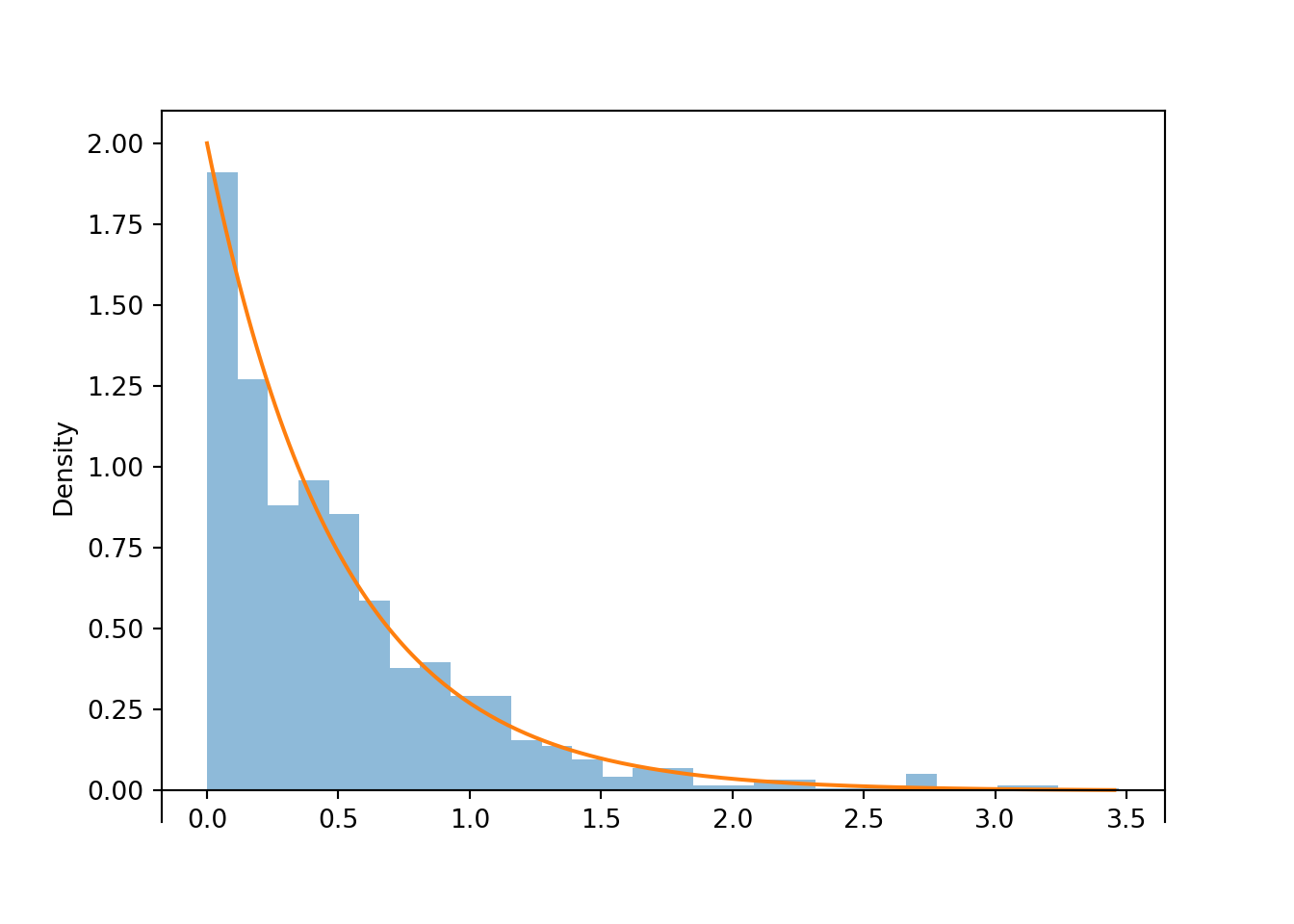

7.1.2 Exponential race

Example 7.6 Xiomara and Rogelio each leave work at noon to meet the other for lunch. The amount of time, $X$, that it takes Xiomara to arrive is a random variable with an Exponential distribution with mean 10 minutes. The amount of time, $Y$, that it takes Rogelio to arrive is a random variable with an Exponential distribution with mean 20 minutes. Assume that $X$ and $Y$ are independent. Let $W$ be the time, in minutes after noon, at which the first person arrives.

What is the relationship between $W$ and $X, Y$?
Find and interpret $\textrm{P}(W>40)$.
Find $\textrm{P}(W > w)$ and identify by name the distribution of $W$.
Find $\textrm{E}(W)$. Is it equal to $\min(\textrm{E}(X), \textrm{E}(Y))$?
Is $\textrm{P}(Y>X)$ greater than or less than 0.5? Make an educated guess for $\textrm{P}(Y > X)$.
Find $\textrm{P}(Y>X|X=10)$.
Find $\textrm{P}(Y>X|X=x)$ for general $x$.
Find $\textrm{P}(Y > X)$. Hint: Use a continuous version of the law of total probability.
Find $\textrm{P}(W>40, Y>X)$.
Find $\textrm{P}(W>w, Y>X)$ for general $w$.
Let $\textrm{I}_{\{Y > X\}}$ be the indicator that Xiomara arrives first. What can you say about $W$ and $\textrm{I}_{\{Y > X\}}$?

Solution. to Example 7.6

Show/hide solution

$W=\min(X, Y)$
Note that $X$ has an Exponential distribution with rate parameter 1/10 (not 10); similarly for $Y$. The earlier arrival time is after 40 minutes if and only if both arrivals occur after 40 minutes: $\{W > 40\}=\{\min(X, Y)>40\} = \{X > 40, Y > 40\}$ \[\begin{align*} \textrm{P}(W > 40) & = \textrm{P}(X > 40, Y > 40) & & \\ & = \textrm{P}(X > 40)\textrm{P}(Y > 40) & & \text{independence}\\ & = e^{-(1/10)(40)}e^{-(1/20)(40)} & & \text{Exponential}\\ & = e^{-(1/10 + 1/20)(40)} = e^{-0.15(40)} = 0.0025 \end{align*}\]
Replace 40 in the previous part with a generic $w>0$. The earlier arrival time is after $w$ minutes if and only if both arrivals occur after $w$ minutes: $\{W > w\}=\{\min(X, Y)>w\} = \{X > w, Y > w\}$ \[\begin{align*} \textrm{P}(W > w) & = \textrm{P}(X > w, Y > w) & & \\ & = \textrm{P}(X > w)\textrm{P}(Y > w) & & \text{independence}\\ & = e^{-(1/10)w}e^{-(1/20)w} & & \text{Exponential}\\ & = e^{-(1/10 + 1/20)w} = e^{-0.15w} \end{align*}\] Therefore, $W$ has an Exponential distribution with rate parameter $1/10 + 1/20 = 0.15$.
Since $W$ has an Exponential(0.15) distribution, $\textrm{E}(W)=1/0.15 = 20/3 = 6.667$ minutes. This is less than $\min(\textrm{E}(X), \textrm{E}(Y)) = \min(10, 20) = 10$. Remember: the expected value of a function is not equal to the function evaluated at the expected value. Taking the smaller of $X, Y$ on a pair-by-pair basis and then averaging yields a smaller value then each of the averages of $X$ and $Y$.
Xiomara has a shorter mean arrival time, so we might expect that she is more likely to arrive first so $\textrm{P}(Y>X)$ should be greater than 0.5. Since on average it takes Rogelio twice as long as Xiomara to arrive, we might expect that Rogelio is twice as likely to be the second person to arrive, so that Xiomara is twice as likely to be the first to arrive. That is, we guess that $\textrm{P}(Y > X)$ is 2/3, and $\textrm{P}(Y < X)$ is 1/3.
Conditioning on $X=10$, treat $X$ like the constant 10. \[\begin{align*} \textrm{P}(Y>X|X=10) & = \textrm{P}(Y > 10 | X = 10) & & \text{Condition on $X=10$} \\ & = \textrm{P}(Y > 10) & & \text{Independence}\\ & = e^{-(1/20)(10)} & & \text{Exponential} \end{align*}\]
For a given $x>0$, conditioning on $X=x$, treat $X$ like the constant $x$. \[\begin{align*} \textrm{P}(Y>X|X=x) & = \textrm{P}(Y > x | X = x) & & \text{Condition on $X=x$} \\ & = \textrm{P}(Y > x) & & \text{Independence}\\ & = e^{-(1/20)x} & & \text{Exponential} \end{align*}\]
The previous part gives the “case by case” probability. Put the cases together to get the overall probability by weighting by the density of each “case”. \[\begin{align*} \textrm{P}(Y > X) & = \int_0^\infty \textrm{P}(Y > X|X=x)f_X(x)dx & & \text{Continuous LOTP}\\ & = \int_0^\infty \left(e^{-(1/20)x}\right) \left(\frac{1}{10}e^{-(1/10)x}\right)dx & & \\ & = \frac{1/10}{1/10 + 1/20} \int_0^\infty \left(1/10 + 1/20\right) \left(e^{-(1/10 + 1/20)x}\right)dx & & \\ & = \frac{1/10}{1/10 + 1/20} = 2/3 & & \end{align*}\]
If $Y>X$ then $W=\min(X, Y) = X$, so $\{W>40, Y>X\}=\{X>40, Y > X\}$. The calculation is similar to the previous part, but not we only integrate over $x>40$. \[\begin{align*} \textrm{P}(W>40, Y > X) & = \int_{40}^\infty \textrm{P}(Y > X|X=x)f_X(x)dx & & \text{Continuous LOTP}\\ & = \int_{40}^\infty e^{-(1/20)x} \left(\frac{1}{10}e^{-(1/10)x}\right)dx & & \\ & = \frac{1/10}{1/10 + 1/20} \int_{40}^\infty \left(1/10 + 1/20\right) \left(e^{-(1/10 + 1/20)x}\right)dx & & \\ & = \frac{1/10}{1/10 + 1/20}e^{-(1/10+1/20)(40)} = (2/3)e^{-0.15(40)} & & \\ & = \textrm{P}(W>40)\textrm{P}(Y > X) & & \end{align*}\]
Replace 40 in the previous part with a generic $w>0$. \[\begin{align*} \textrm{P}(W>w, Y > X) & = \int_{w}^\infty \textrm{P}(Y > X|X=x)f_X(x)dx & & \text{Continuous LOTP}\\ & = \int_{w}^\infty e^{-(1/20)x} \left(\frac{1}{10}e^{-(1/10)x}\right)dx & & \\ & = \frac{1/10}{1/10 + 1/20}e^{-(1/10+1/20)w} = 2/3(e^{-0.15w}) & & \\ & = \textrm{P}(W>w)\textrm{P}(Y > X) & & \end{align*}\]
The previous part shows that the joint distribution of $W$ and $\textrm{I}_{\{Y > X\}}$ factors into the product of their marginal distributions, so $W$ and $\textrm{I}_{\{Y > X\}}$ are independent!


X, Y = RV(Exponential(rate = 1 / 10 ) * Exponential(rate = 1 / 20))

W = (X & Y).apply(min)

(X & Y & W).sim(5)

Index	Result
0	(1.5098839298687947, 16.73093971732583, 1.5098839298687947)
1	(2.320039619321884, 41.019015562479595, 2.320039619321884)
2	(12.386728112422672, 1.0839324356738202, 1.0839324356738202)
3	(55.64543168544119, 0.03237747308983649, 0.03237747308983649)
4	(7.141062796976614, 10.479712806613822, 7.141062796976614)


w = W.sim(10000)
w.plot()

Exponential(rate = 1 / 10 + 1 / 20).plot()
plt.show()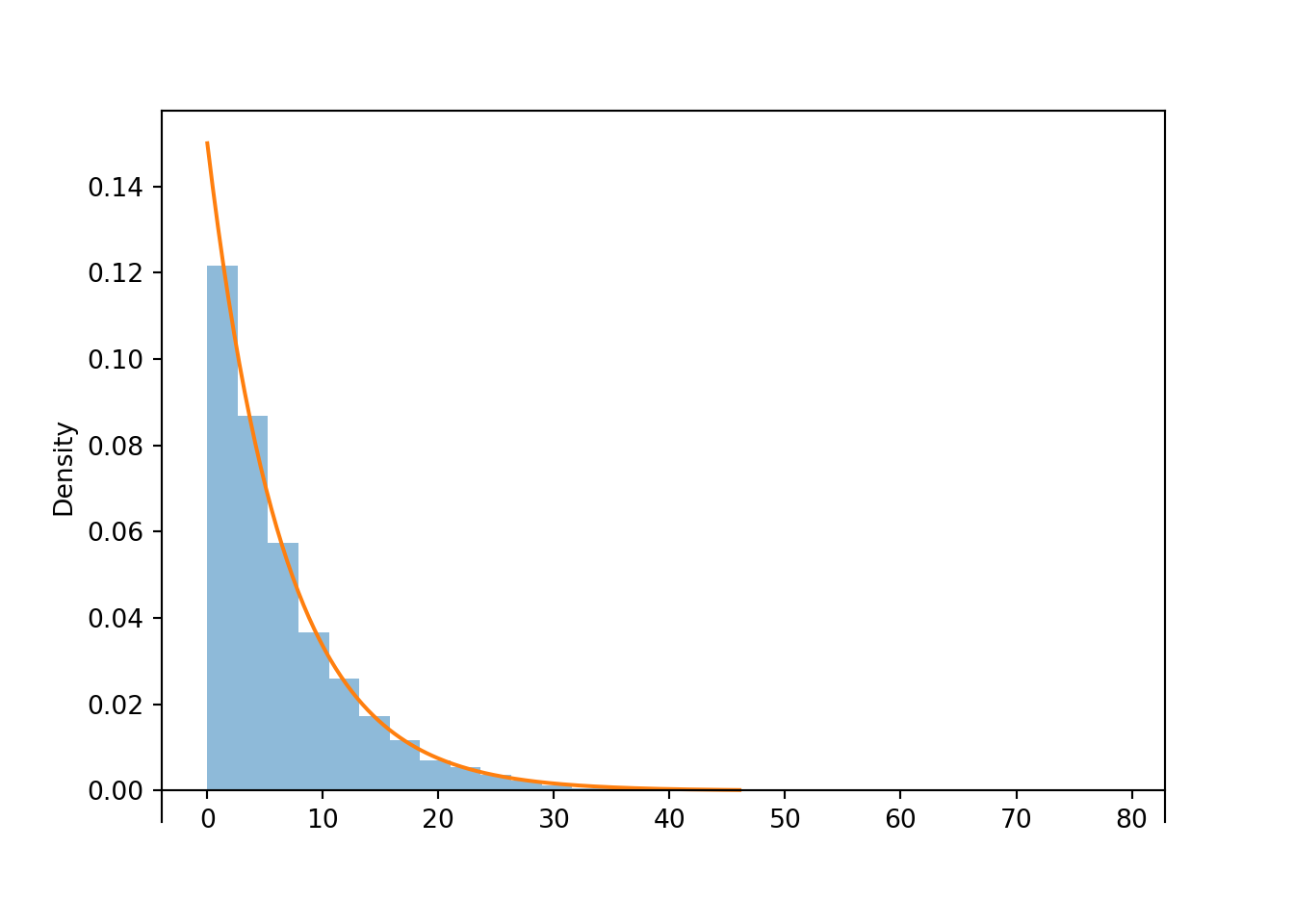


w.mean(), w.sd()

## (6.609110126669045, 6.549951356288915)


(Y > X).sim(10000).tabulate(normalize = True)

Outcome	Relative Frequency
False	0.3335
True	0.6665
Total	1.0


(W | (Y > X) ).sim(10000).plot()
(W | (Y < X) ).sim(10000).plot()

Exponential(rate = 1 / 10 + 1 / 20).plot()
plt.show()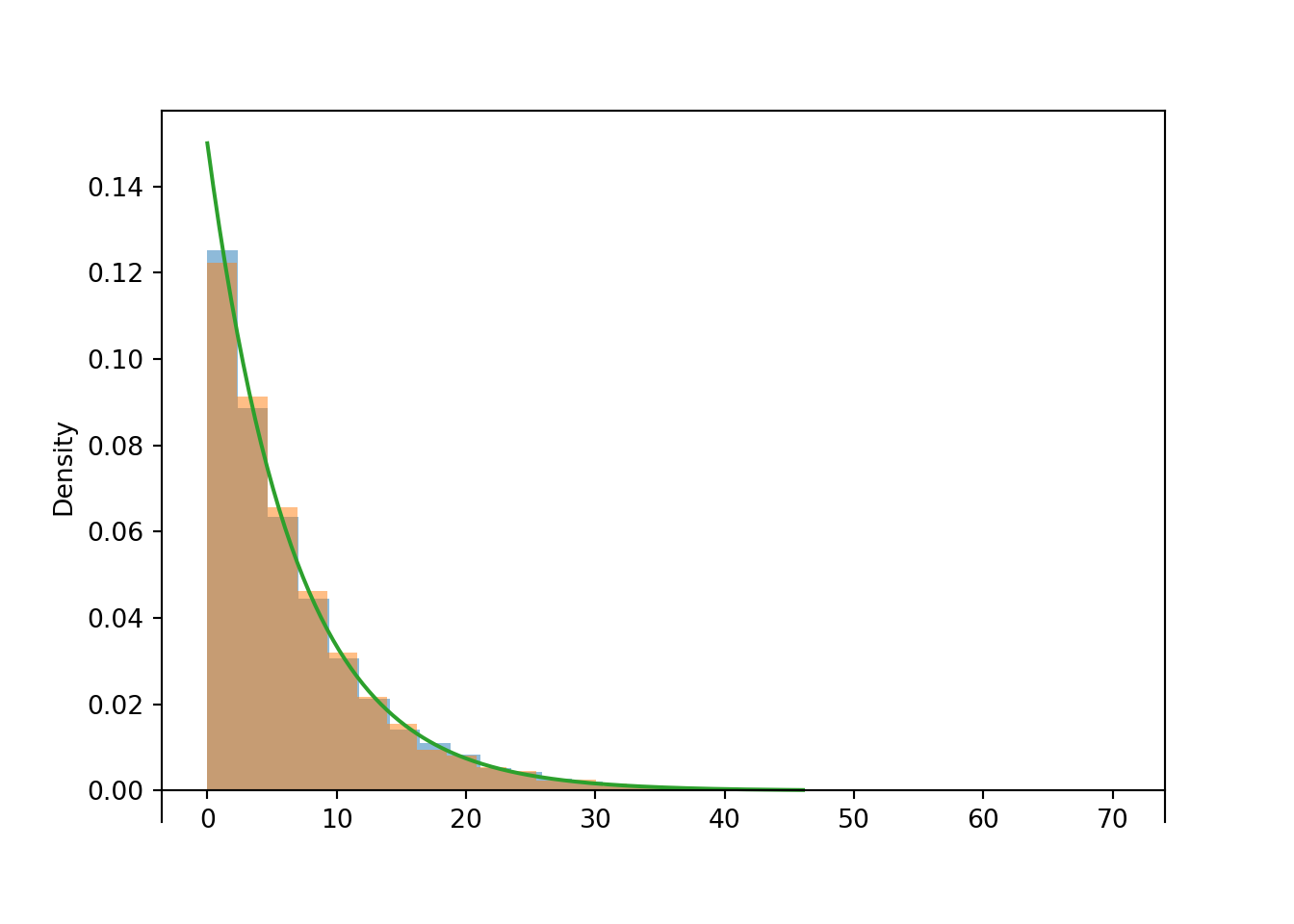

Exponential race (a.k.a., competing risks.) Let $W_1, W_2, \ldots, W_n$ be independent random variables. Suppose $W_i$ has an Exponential distribution with rate parameter $\lambda_i$. Let $W = \min(W_1, \ldots, W_n)$ and let $I$ be the discrete random variable which takes value $i$ when $W=W_i$, for $i=1, \ldots, n$. Then

$W$ has an Exponential distribution with rate $\lambda = \lambda_1 + \cdots+\lambda_n$
$\textrm{P}(I=i) = \textrm{P}(W=W_i) = \frac{\lambda_i}{\lambda_1+\cdots+\lambda_n}, i = 1, \ldots, n$
$W$ and $I$ are independent

Imagine there are $n$ contestants in a race, labeled $1, \ldots, n$, racing independently, and $W_i$ is the time it takes for the $i$th contestant to finish the race. Then $W = \min(W_1, \ldots, W_n)$ is the winning time of the race, and $W$ has an Exponential distribution with rate parameter equal to sum of the individual contestant rate parameters.

The discrete random variable $I$ is the label of which contestant is the winner. The probability that a particular contestant is the winner is the contestant’s rate divided by the total rate. That is, the probability that contestant $i$ is the winner is proportional to the contestant’s rate $\lambda_i$.

Furthermore, $W$ and $I$ are independent. Information about the winning time does not influence the probability that a particular contestant won. Information about which contestant won does not influence the distribution of the winning time.

7.1.3 Gamma distributions

Example 7.7 Suppose that elapsed times (hours) between successive earthquakes are independent, each having an Exponential(2) distribution. Let $T$ be the time elapsed from now until the third earthquake occurs.

Compute $\textrm{E}(T)$.
Compute $\textrm{SD}(T)$.
Does $T$ have an Exponential distribution? Explain.
Use simulation to approximate the distribution of $T$.

Solution. to Example 7.7

Show/hide solution

Let $W_1$ be the elapsed time between now and the first quake, $W_2$ between the first and second, and $W_3$ between the second and third. Then $T=W_1+W_2+W_3$.

$\textrm{E}(T)=\textrm{E}(W_1+W_2+W_3) = \textrm{E}(W_1)+\textrm{E}(W_2)+\textrm{E}(W_3) = 3(1/2)$.
Since the $W_i$s are independent, $\textrm{Var}(T)=\textrm{Var}(W_1+W_2+W_3) = \textrm{Var}(W_1)+\textrm{Var}(W_2)+\textrm{Var}(W_3) = 3(1/4)$. So $\textrm{SD}(T)=\sqrt{3}(1/2)$.
$T$ does not have an Exponential distribution. For an Exponential distribution, the mean and the SD are the same, but here $\textrm{E}(T)\neq \textrm{SD}(T)$.
See the simulation results below. We see that the distribution is not Exponential.


W1, W2, W3 = RV(Exponential(rate = 2) ** 3)

T = W1 + W2 + W3

T.sim(10000).plot()

Gamma(3, rate = 2).plot()
plt.show()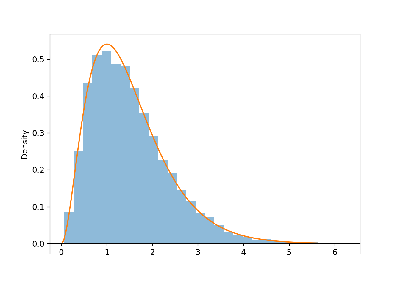

Definition 7.2 A continuous random variable $X$ has a Gamma distribution with shape parameter $\alpha$, a positive integer¹³⁸, and rate parameter¹³⁹ $\lambda>0$ if its pdf is \[\begin{align*} f_X(x) & = \frac{\lambda^\alpha}{(\alpha-1)!} x^{\alpha-1}e^{-\lambda x} , & x \ge 0,\\ & \propto x^{\alpha-1}e^{-\lambda x} , & x \ge 0 \end{align*}\] If $X$ has a Gamma($\alpha$, $\lambda$) distribution then \[\begin{align*} \textrm{E}(X) & = \frac{\alpha}{\lambda}\\ \textrm{Var}(X) & = \frac{\alpha}{\lambda^2}\\ \textrm{SD}(X) & = \frac{\sqrt{\alpha}}{\lambda} \end{align*}\]

If $W_1, \ldots, W_n$ are independent and each $W_i$ has an Exponential($\lambda$) distribution then $(W_1+\cdots+W_n)$ has a Gamma($n$,$\lambda$) distribution. Each $W_i$ represents the waiting time between two occurrences of some event, so $W_1 + \cdots+ W_n$ represents the total waiting time until a total of $n$ occurrences.

Exponential distributions are continuous analogs of Geometric distributions, and Gamma distributions are continuous analogs of Negative Binomial distributions.

For a positive integer $d$, the Gamma($d/2, 1/2$) distribution is also known as the chi-square distribution with $d$ degrees of freedom.

Here’s a useful fact: $\int_0^\infty u^{k}e^{-u} du = k!$, for any nonnegative integer $k$.↩︎
Exponential distributions are sometimes parametrized directly by their mean $1/\lambda$, instead of the rate parameter $\lambda$. The mean $1/\lambda$ is called the scale parameter.↩︎
Geometric distributions are the only discrete distributions with the discrete analog of the memoryless property.↩︎
There is a more general expression of the pdf which replaces $(\alpha-1)!$ with the Gamma function $\Gamma(\alpha)=\int_0^\infty u^{\alpha-1}e^{-u} du$, that can be used to define a Gamma pdf for any $\alpha>0$. When $\alpha$ is a positive integer, $\Gamma(\alpha)=(\alpha-1)!$.↩︎
Like Exponential distributions, Gamma distributions are sometimes parametrized directly by their mean $1/\lambda$, instead of the rate parameter $\lambda$. The mean $1/\lambda$ is called the scale parameter.↩︎