4.9 Independence of random variables
Example 4.45 Suppose \(X\) and \(Y\) are random variables whose joint pmf is represented by the following table.
| \(p_{X, Y}(x, y)\) | |||||
|---|---|---|---|---|---|
| \(x\) \ \(y\) | 1 | 2 | 3 | \(p_X(x)\) | |
| 0 | 0.20 | 0.50 | 0.10 | 0.80 | |
| 1 | 0.05 | 0.10 | 0.05 | 0.20 | |
| \(p_Y(y)\) | 0.25 | 0.60 | 0.15 |
- Are the events \(\{X=0\}\) and \(\{Y=1\}\) independent?
- Are the random variables \(X\) and \(Y\) are independent? Why?
- What would the joint pmf need to be in order for random variables with these marginal pmfs to be independent?
Solution. to Example 4.45
Show/hide solution
Yes. \(\textrm{P}(X=0, Y=1) = p_{X, Y}(0, 1) = 0.20 = (0.80)(0.25) = p_X(0)p_Y(1) = \textrm{P}(X=0)\textrm{P}(Y=1)\).
No. In particular, \(\textrm{P}(X = 0) = 0.8\), but \(\textrm{P}(X = 0|Y=3) = 0.10/0.15 = 2/3\). Knowing the value of one of the variables changes the distribution of the other.
We need each joint probability to be the product of the corresponding marginal probability as in part 1.
\(p_{X, Y}(x, y)\) \(x\) \ \(y\) 1 2 3 \(p_X(x)\) 0 0.20 0.48 0.12 0.80 1 0.05 0.12 0.03 0.20 \(p_Y(y)\) 0.25 0.60 0.15
Definition 4.13 Two random variables \(X\) and \(Y\) defined on a probability space with probability measure \(\textrm{P}\) are independent if \(\textrm{P}(X\le x, Y\le y) = \textrm{P}(X\le x)\textrm{P}(Y\le y)\) for all \(x, y\). That is, two random variables are independent if their joint cdf is the product of their marginal cdfs.
Random variables \(X\) and \(Y\) are independent if and only if the joint distribution factors into the product of the marginal distributions. The definition is in terms of cdfs, but analogous statements are true for pmfs and pdfs. Intuitively, random variables \(X\) and \(Y\) are independent if and only if the conditional distribution of one variable is equal to its marginal distribution regardless of the value of the other.
Discrete random variables are independent if and only if the joint pmf is the product of the marginal pmfs, and if and only if the conditional pmfs are equal to the corresponding marginal pmfs. For discrete random variables \(X\) and \(Y\), the following are equivalent.
\[\begin{align*} \text{Discrete RVs $X$ and $Y$} & \text{ are independent}\\ \Longleftrightarrow p_{X,Y}(x,y) & = p_X(x)p_Y(y) & & \text{for all $x,y$}\\ \Longleftrightarrow p_{X|Y}(x|y) & = p_X(x) & & \text{for all $x,y$} \\ \Longleftrightarrow p_{Y|X}(y|x) & = p_Y(y) & & \text{for all $x,y$} \end{align*}\]
Continuous random variables are independent if and only if the joint pdf is the product of the marginal pdfs, and if and only if the conditional pdfs are equal to the corresponding marginal pdfs. For continuous random variables \(X\) and \(Y\), the following are equivalent.
\[\begin{align*} \text{Continuous RVs $X$ and $Y$} & \text{ are independent}\\ \Longleftrightarrow f_{X,Y}(x,y) & = f_X(x)f_Y(y) & & \text{for all $x,y$}\\ \Longleftrightarrow f_{X|Y}(x|y) & = f_X(x) & & \text{for all $x,y$} \\ \Longleftrightarrow f_{Y|X}(y|x) & = f_Y(y) & & \text{for all $x,y$} \end{align*}\]
If \(X\) and \(Y\) are independent, then the (renormalized) distributions of \(Y\) values along each \(X\)-slice have the same shape as each other, and the same shape as the marginal distribution of \(Y\). Likewise, If \(X\) and \(Y\) are independent, then the (renormalized) distributions of \(X\) values along each \(Y\)-slice have the same shape as each other, and the same shape as the marginal distribution of \(X\).
Example 4.46 Recall Example 4.32. Let \(X\) be the number of home runs hit by the home team, and \(Y\) the number of home runs hit by the away team in a randomly selected MLB game. Suppose that \(X\) and \(Y\) have joint pmf
\[ p_{X, Y}(x, y) = \begin{cases} e^{-2.3}\frac{x^{1.2}y^{1.1}}{x!y!}, & x = 0, 1, 2, \ldots; y = 0, 1, 2, \ldots,\\ 0, & \text{otherwise.} \end{cases} \]
The marginal pmf of \(X\) is \[ p_{X}(x) = e^{-1.2}\frac{x^{1.2}}{x!},\quad x = 0, 1, 2, \ldots \]
The marginal pmf of \(Y\) is \[ p_{Y}(y) = e^{-1.1}\frac{y^{1.1}}{y!},\quad y = 0, 1, 2, \ldots \]
- Find the probability that the home teams hits 2 home runs.
- Are \(X\) and \(Y\) independent? (Note: we’re asking about independence in terms of the assumed probability model, not for your opinion based on your knowledge of baseball.)
- Find the probability that the home teams hits 2 home runs and the away team hits 1 home run.
- Find the probability that the home teams hits 2 home runs given the away team hits 1 home run.
- Find the probability that the home teams hits 2 home runs given the away team hits at least 1 home run.
Solution. to Example 4.46
Show/hide solution
- Use the marginal pmf of \(X\). \(\textrm{P}(X = 2) = p_{X}(2) =e^{-1.2}\frac{1.2^2}{2!}=0.217\).
- Yes, the joint pmf is the product of the marginal pmfs.
- Since \(X\) and \(Y\) are independent \(\textrm{P}(X = 2, Y = 1) = p_{X, Y}(2, 1) = p_{X}(2)p_{Y}(1) = e^{-1.2}\frac{1.2^2}{2!}e^{-1.1}\frac{1.1^1}{1!}= 0.0794\).
- Since \(X\) and \(Y\) are independent \(\textrm{P}(X = 2|Y = 1) = \textrm{P}(X = 2) = p_{X}(2) =e^{-1.2}\frac{1.2^2}{2!}= 0.217\).
- Since \(X\) and \(Y\) are independent \(\textrm{P}(X = 2|Y \ge 1) = \textrm{P}(X = 2) = p_{X}(2) =e^{-1.2}\frac{1.2^2}{2!}= 0.217\).
Are home and away team home runs in baseball games really independent? Compare Figured 4.43 and 4.44. The mosaic plot in Figure 4.43 represents Example 4.46 in which \(X\) and \(Y\) are assumed to be independent.
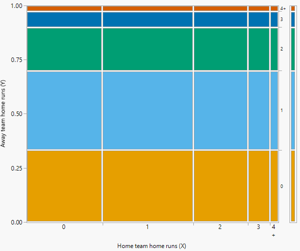
Figure 4.43: Mosaic plot for Example 4.46 where \(X\) and \(Y\) are assumed to be independent. The plot represents conditioning on the value of home team home runs, \(X\). The colors represent different values of away team home runs, \(Y\).
Let’s compare with some real data. The mosaic plot in Figure 4.44 is based on actual home run data from the 2018 MLB season. While there is not an exact match, the model from Example 4.46 seems to describe the data reasonably well. In particular, there does not appear to be much dependence between home runs hit by the two teams in a game.
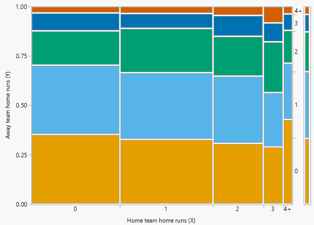
Figure 4.44: Mosaic plot based on home run data from the 2018 MLB season. The plot represents conditioning on the value of home team home runs, \(X\). The colors represent different values of away team home runs, \(Y\).
Example 4.47 Let \(X\) and \(Y\) be continuous random variables with joint pdf
\[ f_{X, Y}(x, y) = e^{-x}, \qquad x>0,\; 0<y<1. \]
- Without doing any calculations, find the conditional distributions and marginal distributions.
- Are \(X\) and \(Y\) independent?
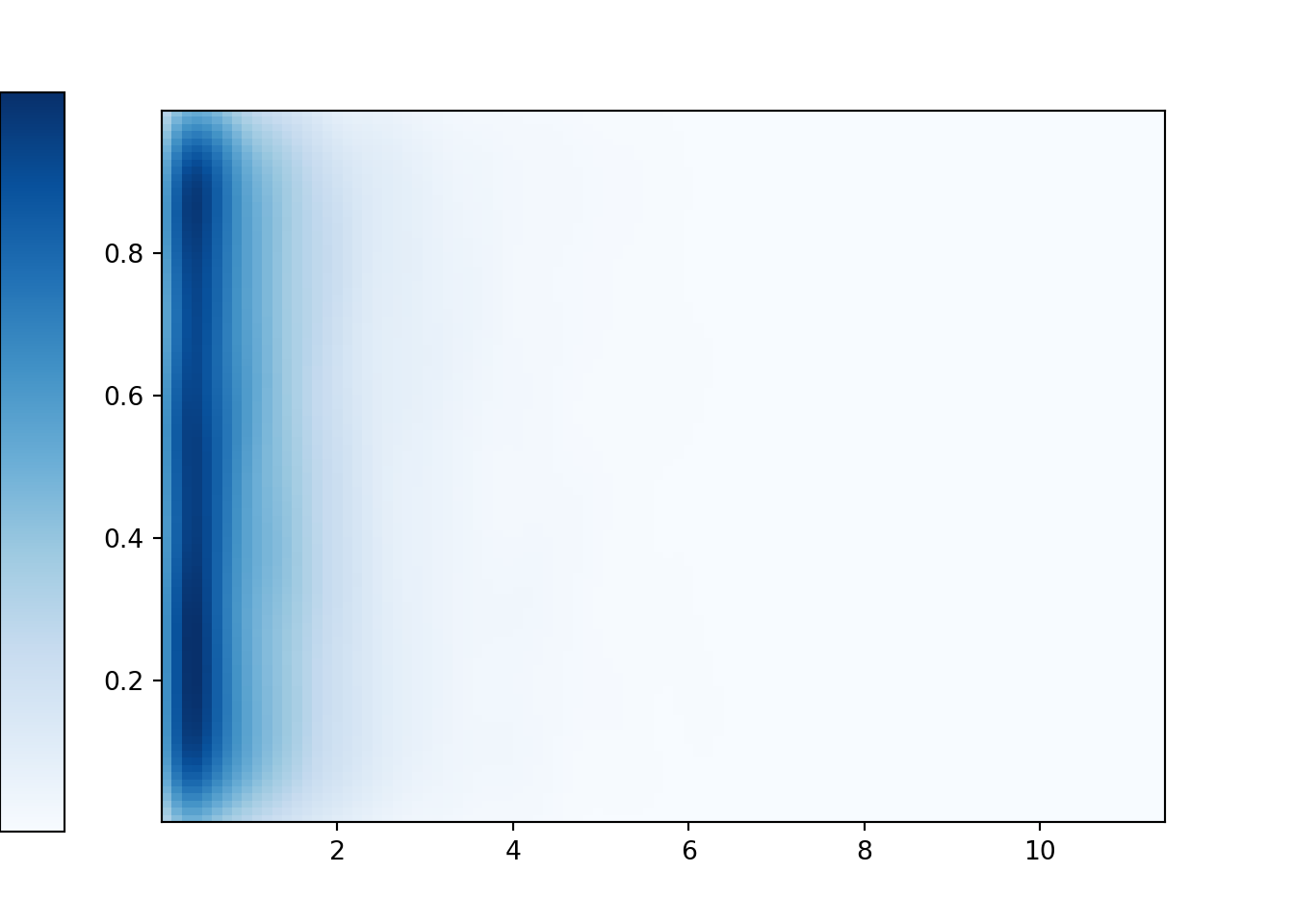
- Sketch a plot of the joint pdf of \(X\) and \(Y\).
- Find \(\textrm{P}(X<0.2, Y<0.4)\).
- Find \(\textrm{P}(X<0.2| Y<0.4)\).
Solution. to Example 4.47
Show/hide solution
- Fix \(y\). Then as a function of \(x\), the conditional pdf of \(X\) given \(Y=y\) is proportional to \(e^{-x}, x>0\). That is true for any \(0<y<1\). So regardless of the value of \(Y\), \(X\) follows an Exponential(1) distribution. Now fix \(x\). Regardless of the value of \(x\), the conditional pdf of \(Y\) given \(X=x\) is constant over the (0, 1) range of possible \(y\) values. That is, regardless of the value of \(X\), \(Y\) follows a Uniform(0, 1) distribution.
- Yes, because of the previous part. The joint pdf factors in the product of marginal pdfs. By carefully inspecting the joint pdf, we can determine, without any calculations, that \(X\) and \(Y\) are independent, \(X\) has a marginal Exponential(1) distribution, and \(Y\) has a Uniform(0, 1) distribution.
- See the simulation results below. Each vertical slice, corresponding to the distribution of values of \(Y\) for a given value of \(X\), has constant Uniform(0, 1) density. Each horizontal slice, corresponding to the distribution of values of \(X\) for a given value of \(Y\), has an Exponential(1) density.
- \(X\) and \(Y\) are independent so \(\textrm{P}(X<0.2, Y<0.4)=\textrm{P}(X<0.2)\textrm{P}(Y<0.4) = (1-e^{-0.2})(0.4)=0.073\).
- \(X\) and \(Y\) are independent so \(\textrm{P}(X<0.2| Y<0.4)=\textrm{P}(X<0.2) = 1-e^{-0.2}=0.181\).
Continuous random variables \(X\) and \(Y\) are independent if and only if their joint pdf can be factored into the product of a function of values of \(X\) alone and a function of values of \(Y\) alone. That is, \(X\) and \(Y\) are independent if and only if there exist functions \(g\) and \(h\) for which \[ f_{X,Y}(x,y) \propto g(x)h(y) \qquad \text{ for all $x$, $y$} \] Aside from normalizing constants, \(g\) determines the shape of the marginal pdf for \(X\), and \(h\) for \(Y\). Be careful: when determining if the pdfs can be factored, be sure to consider the range of possible \(x\) and \(y\) values. Random variables are not independent if the possible values of one variable can change given the value of the other.
If \(X\) and \(Y\) are independent then the joint pdf factors into a product of the marginal pdfs. The above result says that if the joint pdf factors into two separate factors — one involving values of \(X\) alone, and one involving values of \(Y\) alone — then \(X\) and \(Y\) are independent. The above result is useful because it allows you to determine whether \(X\) and \(Y\) are independent without first finding their marginal distributions.
Some Symbulate code for Example 4.47 follows. We can define two independent random variables by specifying their joint distribution as the product * of their marginal distributions.
X, Y = RV(Exponential(1) * Uniform(0, 1))

plt.figure()
(X & Y).sim(10000).plot('density')
plt.show()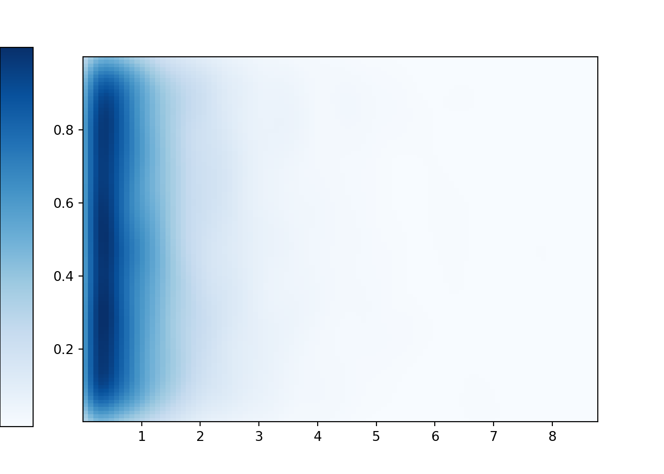
We can also simulate conditional distributions. Remember: be careful when conditioning on the value of a continuous random variable.
plt.figure()
(X | (abs(Y - 0.1) < 0.05) ).sim(1000).plot(bins = 20) # given Y "=" 0.1
(X | (abs(Y - 0.5) < 0.05) ).sim(1000).plot(bins = 20) # given Y "=" 0.5
(X | (abs(Y - 0.7) < 0.05) ).sim(1000).plot(bins = 20) # given Y "=" 0.7
plt.show()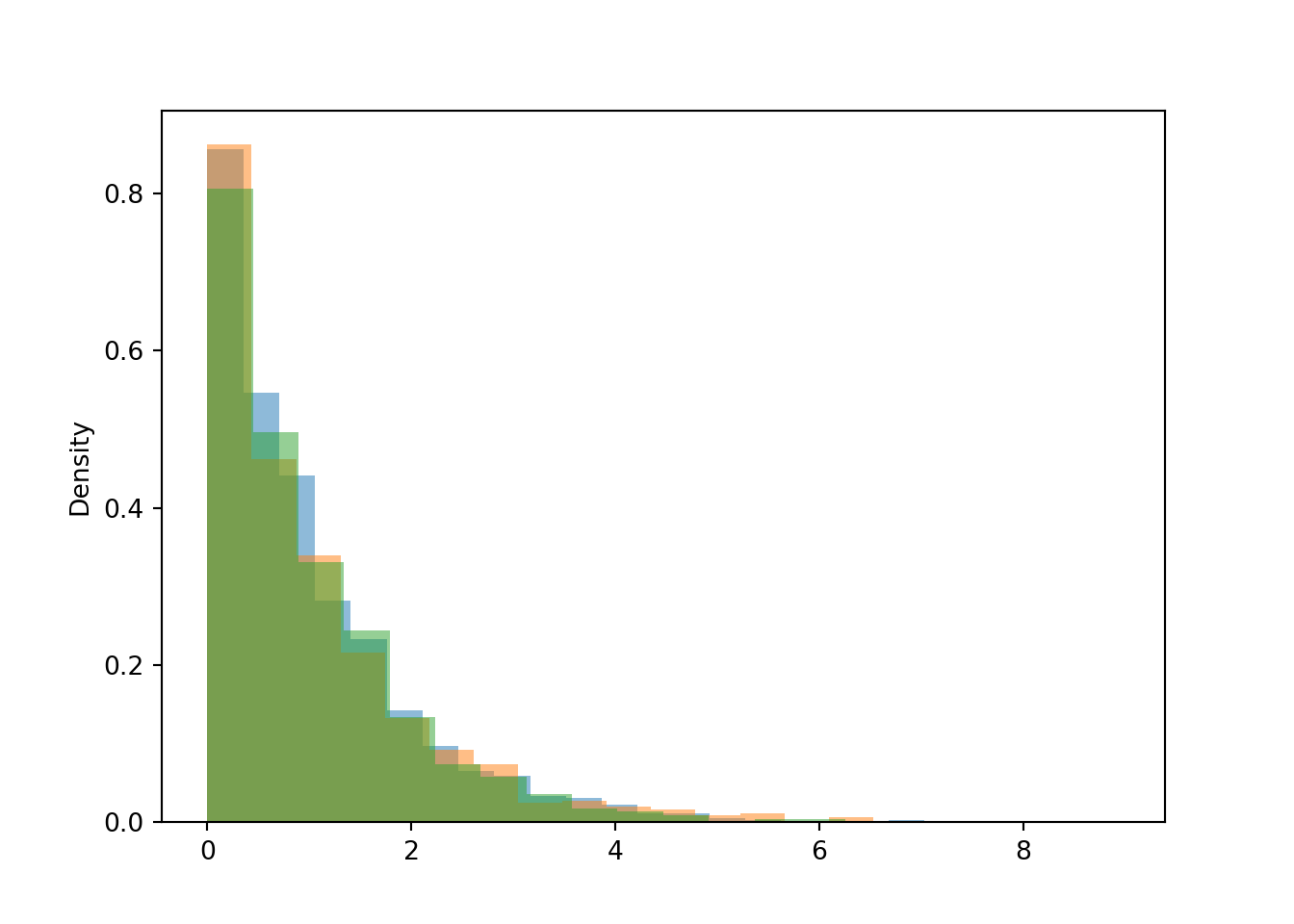
plt.figure()
(Y | (abs(X - 0.1) < 0.05) ).sim(1000).plot(bins = 20) # given X "=" 0.1
(Y | (abs(X - 0.5) < 0.05) ).sim(1000).plot(bins = 20) # given X "=" 0.5
(Y | (abs(X - 0.7) < 0.05) ).sim(1000).plot(bins = 20) # given X "=" 0.7
plt.show()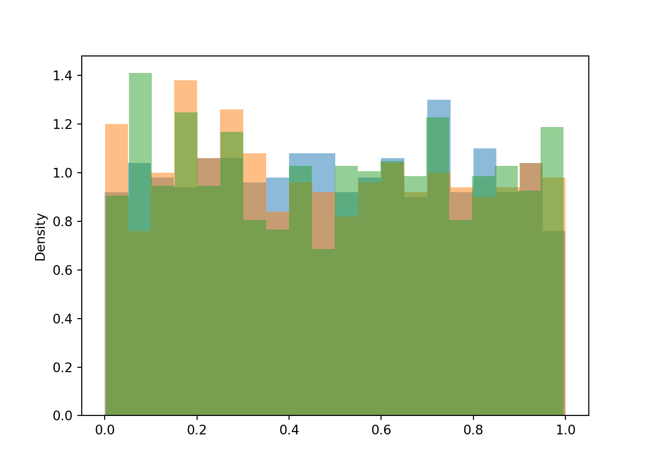
Donny Dont wants to code this example in Symbulate as
X = RV(Exponential(1))
Y = RV(Uniform(0, 1))
Unfortunately, the above code returns an error when attempting (X & Y).sim(1000). The reason is that the above code only specifies the marginal distributions of \(X\) and \(Y\), but the joint distribution is needed to generate \((X, Y)\) pairs. If you want \(X\) and \(Y\) to be independent, you need to make that explicit. One way to fix Donny’s code is to add a line which tells Symbulate that \(X\) and \(Y\) are independent, in which case it is enough to specify the marginal distributions.
X = RV(Exponential(1))
Y = RV(Uniform(0, 1))

X, Y = AssumeIndependent(X, Y)

plt.figure()
(X & Y).sim(10000).plot('density')
plt.show()