4.1 Do not confuse a random variable with its distribution
Heed the title. A random variable measures a numerical quantity which depends on the outcome of a random phenomenon. The distribution of a random variable specifies the long run pattern of variation of values of the random variable over many repetitions of the underlying random phenomenon. The distribution of a random variable can be approximated by simulating an outcome of the random process, observing the value of the random variable for that outcome, repeating this process many times, and summarizing the results. But a random variable is not its distribution.
A distribution is determined by:
- The underlying probability measure \(\textrm{P}\), which represents all the assumptions about the random phenomenon.
- The random variable \(X\) itself, that is, the function which maps sample space outcomes to numbers.
Changing either the probability measure or the random variable itself can change the distribution of the random variable. For example, consider the sample space of two rolls of a fair four-sided die. In each of the following scenarios, the random variable \(X\) has a different distribution.
- The die is fair and \(X\) is the sum of the two rolls
- The die is fair and \(X\) is the larger of the two rolls
- The die is weighted to land on 1 with probability 0.1 and 4 with probability 0.4 and \(X\) is the sum of the two rolls.
In particular, in (1) \(X\) takes the value 2 with probability \(1/16\), in (2) \(X\) takes the value 2 with probability \(3/16\), and in (3) \(X\) takes the value 2 with probability 0.01. In (1) and (2), the probability measure is the same (fair die) but the function defining the random variable is different (sum versus max). In (1) and (3), the function defining the random variable is the same, and the sample space of outcomes is the same, but the probability measure is different.
We often specify the distribution of a random variable directly without explicit mention of the underlying probability space or function defining the random variable. For example, in the meeting problem we might assume that arrival times follow a Uniform(0, 60) or a Normal(30, 10) distribution. In situations like this, you can think of the probability space as being the distribution of the random variable and the function defining the random variable to be the identity function. This idea corresponds to the “simulate from the distribution method”: construct a spinner corresponding to the distribution of the random variable and spin it to simulate a value of the random variable.
Example 4.1 Donny Dont is thoroughly confused about the distinction between a random variable and its distribution. Help him understand by by providing a simple concrete example of two different random variables \(X\) and \(Y\) that have the same distribution. Can you think of \(X\) and \(Y\) for which \(\textrm{P}(X = Y) = 0\)? How about a discrete example and a continuous example?
Solution. to Example 4.1
Show/hide solution
Flip a fair coin 3 times and let \(X\) be the number of heads and \(Y\) be the number of tails. Then \(X\) and \(Y\) have the same distribution, because they have the same long run pattern of variability. Each variable takes values 0, 1, 2, 3 with probability 1/8, 3/8, 3/8, 1/8. But they are not the same random variable; they are measuring different things. If the outcome is HHT then \(X\) is 2 but \(Y\) is 1. In this case \(\textrm{P}(X = Y)=0\); in an odd number of flips it’s not possible to have the same number of heads and tails on any single outcome.
In some cases of the meeting time problem we assumed the distribution of Regina’s arrival time \(R\) is Uniform(0, 60) and the distribution of Cady’s arrival time \(Y\) is Uniform(0, 60). So \(R\) and \(Y\) have the same distribution. But these are two random variables; one measures Regina’s arrival time and one measure Cady’s. If Regina and Cady met every day for a year, then the day-to-day pattern of Regina’s arrival times would look like the day-to-day pattern of Cady’s arrival times. But on any given day, their arrival times would not be the same, since \(R\) and \(Y\) are continuous random variables so \(\textrm{P}(R = Y) = 0\).
A distribution, like a spinner, is a blueprint for simulating values of the random variable. If two random variables have the same distribution, you could use the same spinner to simulate values of either random variable. But a distribution is not the random variable itself. (In other words, “the map is not the territory.”)
Two random variables can have the same (long run) distribution, even if the values of the two random variables are never equal on any particular repetition (outcome). If \(X\) and \(Y\) have the same distribution, then the spinner used to simulate \(X\) values can also be used to simulate \(Y\) values; in the long run the patterns would be the same.
At the other extreme, two random variables \(X\) and \(Y\) are the same random variable only if for every outcome of the random phenomenon the resulting values of \(X\) and \(Y\) are the same. That is, \(X\) and \(Y\) are the same random variable only if they are the same function: \(X(\omega)=Y(\omega)\) for all \(\omega\in\Omega\). It is possible to have two random variables for which \(\textrm{P}(X=Y)\) is large, but \(X\) and \(Y\) have different distributions.
Many commonly encountered distributions have special names. For example, the distribution of \(X\), the number of heads in 3 flips of a fair coin, is called the “Binomial(3, 0.5)” distribution. If a random variable has a Binomial(3, 0.5) distribution then it takes the possible values 0, 1, 2, 3, with respective probability 1/8, 3/8, 3/8, 1/8. The random variable in each of the following situations has a Binomial(3, 0.5) distribution.
- \(Y\) is the number of Tails in three flips of a fair coin
- \(Z\) is the number of even numbers rolled in three rolls of a fair six-sided die
- \(W\) is the number of female babies in a random sample of three births at a hospital (assuming boys and girls are equally likely99)
Each of these situations involves a different sample space of outcomes (coins, dice, births) with a random variable which counts different things (Heads, Tails, evens, boys). But all the scenarios have some general features in common:
- There are 3 “trials” (3 flips, 3 rolls, 3 babies)
- Each trial can be classified as “success”100 (Tails, even, female) or “failure”.
- Each trial is equally likely to result in success or not (fair coin, fair die, assuming boys and girls are equally likely)
- The trials are independent. For coins and dice the trials are physically independent. For births independence follows from random selection from a large population.
- The random variable counts the number of successes in the 3 trials (number of T, number of even rolls, number of female babies).
These examples illustrate that knowledge that a random variable has a specific distribution (e.g., Binomial(3, 0.5)) does not necessarily convey any information about the underlying outcomes or random variable (function) being measured. (We will study Binomial distributions in more detail later.)
The scenarios involving \(W, X, Y, Z\) illustrate that two random variables do not have to be defined on the same sample space in order to determine if they have the same distribution. This is in contrast to computing quantities like \(\textrm{P}(X=Y)\): \(\{X=Y\}\) is an event which cannot be investigated unless \(X\) and \(Y\) are defined for the same outcomes. For example, you could not estimate the probability that a student has the same score on both SAT Math and Reading exams unless you measured pairs of scores for each student in a sample. However, you could collect SAT Math scores for one set of students to estimate the marginal distribution of Math scores, and collect Reading scores for a separate set of students to estimate the marginal distribution of Reading scores.
A random variable can be defined explicitly as a function on a probability space, or implicitly through its distribution.
The distribution of a random variable is often assumed or specified directly, without mention of the underlying probabilty space or the function defining the random variable.
For example, a problem might state “let \(Y\) have a Binomial(3, 0.5) distribution” or “let \(Y\) have a Normal(30, 10) distribution”.
But remember, such statements do not necessarily convey any information about the underlying sample space outcomes or random variable (function) being measured.
In Symbulate the RV command can also be used to define a RV implicitly via its distribution.
A definition like X = RV(Binomial(3, 0.5)) effectively defines a random variable X on an unspecified probability space via an unspecified function.
W = RV(Binomial(3, 0.5))

plt.figure()
W.sim(10000).plot()
plt.show()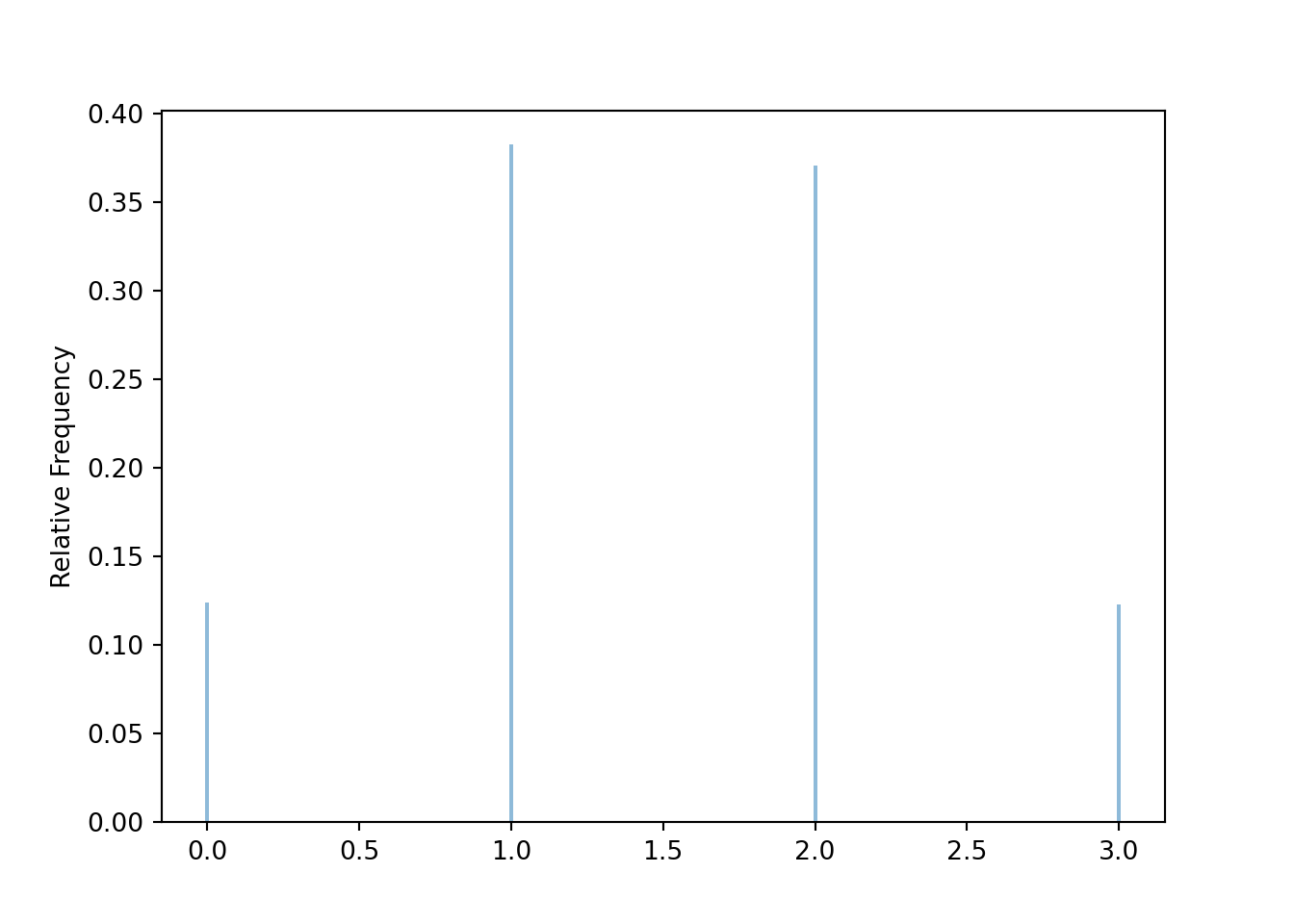
Example 4.2 Suppose that \(X\), \(Y\), and \(Z\) all have the same distribution. Donny Dont says
- The pair \((X, Y)\) has the same joint distribution as the pair \((X, Z)\).
- \(X+Y\) has the same distribution as \(X+Z\).
- \(X+Y\) has the same distribution as \(X+X=2X\).
Determine if each of Donny’s statements is correct. If not, explain why not using a simple example.
Solution. to Example 4.2
Show/hide solution
First of all, Donny’s statements wouldn’t even make sense unless the random variables were all defined on the same probability space. For example, if \(X\) is SAT Math score and \(Y\) is SAT reading score it doesn’t makes sense to consider \(X+Y\) unless \((X, Y)\) pairs are measured for the same students. But even assuming the random variables are defined on the same probability space, we can find counterexamples to Donny’s statements.
As just one example, flip a fair coin 4 times and let
- \(X\) be the number of heads in flips 1 through 3
- \(Y\) be the number of tails in flips 1 through 3
- \(Z\) be the number of heads in flips 2 through 4.
- The joint distribution of \((X, Y)\) is not the same as the joint distribution of \((X, Z)\). For example, \((X, Y)\) takes the pair \((3, 3)\) with probability 0, but \((X, Z)\) takes the pair \((3, 3)\) with nonzero probability (1/16).
- The distribution of \(X+Y\) is not the same as the distribution of \(X+Z\); \(X+Y\) is 3 with probability 1, but the probability that \(X+Z\) is 3 is less than 1 (4/16).
- The distribution of \(X+Y\) is not the same as the distribution of \(2X\); \(X+Y\) is 3 with probability 1, but \(2X\) takes values 0, 2, 4, 6 with nonzero probability.
Remember that a joint distribution is a probability distribution on pairs of values. Just because \(X_1\) and \(X_2\) have the same marginal distribution, and \(Y_1\) and \(Y_2\) have the same marginal distribution, doesn’t necessary imply that \((X_1, Y_1)\) and \((X_2, Y_2)\) have the same joint distributions. In general, information about the marginal distributions alone is not enough to determine information about the joint distribution. We saw a related two-way table example in Section 2.8. Just because two two-way tables have the same totals, they don’t necessarily have the same interior cells.
The distribution of any random variable obtained via a transformation of multiple random variables will depend on the joint distribution of the random variables involved; for example, the distribution of \(X+Y\) depends on the joint distribution of \(X\) and \(Y\).
Example 4.3 Consider the probability space corresponding to two spins of the Uniform(0, 1) spinner and let \(U_1\) be the result of the first spin and \(U_2\) the result of the second. For each of the following pairs of random variables, determine whether or not they have the same distribution as each other. No calculations necessary; just think conceptually.
- \(U_1\) and \(U_2\)
- \(U_1\) and \(1-U_1\)
- \(U_1\) and \(1+U_1\)
- \(U_1\) and \(U_1^2\)
- \(U_1+U_2\) and \(2U_1\)
- \(U_1\) and \(1-U_2\)
- Is the joint distribution of \((U_1, 1-U_1)\) the same as the joint distribution of \((U_1, 1 - U_2)\)?
Solution. to Example 4.3
Show/hide solution
- Yes, each has a Uniform(0, 1) distribution.
- Yes, each has a Uniform(0, 1) distribution. For \(u\in[0, 1]\), \(1-u\in[0, 1]\), so \(U_1\) and \(1-U_1\) have the same possible values, and a linear rescaling does not change the shape of the distribution. Changing from \(U_1\) to \(1-U_1\) essentially amounts to switching the [0, 1] labels on the spinner from clockwise to counterclockwise.
- No, the two variables do not have the same possible values. The shapes would be similar though; \(1+U_1\) has a Uniform(1, 2) distribution.
- No, a non-linear rescaling generally changes the shape of the distribution. For example, \(\textrm{P}(U_1\le0.49) = 0.49\), but \(\textrm{P}(U_1^2 \le 0.49) = \textrm{P}(U_1 \le 0.7) = 0.7\) Squaring a number in [0, 1] makes the number even smaller, so the distribution of \(U_1^2\) places higher density on smaller values than \(U_1\) does.
- No, \(U_1+U_2\) has a triangular shaped distribution on (0, 2) with a peak at 1. (The shape is similar to that of the distribution of \(X\) in Section ??, but the possible values are (0, 2) rather than (2, 8).) But \(2U_1\) has a Uniform(0, 2) distribution. Do not confuse a random variable with its distribution. Just because \(U_1\) and \(U_2\) have the same distribution, you cannot replace \(U_2\) with \(U_1\) in transformations. The random variable \(U_1+U_2\) is not the same random variable as \(2U_1\); spinning a spinner and adding the spins will not necessarily produce the same value as spinner a spinner once and multiplying the value by 2.
- Yes, just like \(U_1\) and \(1-U_2\) have the same distribution.
- No. The marginal distributions are the same, but the joint distribution of \((U_1, 1-U_1)\) places all density along a line, while the joint density of \((U_1, 1-U_2)\) is distributed over the whole two-dimensional region \([0, 1]\times[0,1]\).
Do not confuse a random variable with its distribution. This is probably getting repetitive by now, but we’re emphasizing this point for a reason. Many common mistakes in probability problems involve confusing a random variable with its distribution. For example, we will soon that if a continuous random variable \(X\) has probability density function \(f(x)\), then the probability density function of \(X^2\) is NOT \(f(x^2)\) nor \((f(x))^2\). Mistakes like these, which are very common, essentially involve confusing a random variable with its distribution. Understanding the fundamental difference between a random variable and its distribution will help you avoid many common mistakes, especially in problems involving a lot of calculus or mathematical symbols.
There is no value judgment; sSuccess” just refers to whatever we’re counting. Did the thing we’re counting happen on this trial (“success) or not (”failure”). Success isn’t necessarily good.↩︎