2.11 Joint distributions

Most interesting problems involve two or more⁸³ random variables defined on the same probability space. In these situations, we can consider how the variables vary together, or jointly, and study their relationship. The joint distribution of random variables $X$ and $Y$ (defined on the same probability space) is a probability distribution on $(x, y)$ pairs. (Remember that he distribution of one of the variables alone is a “marginal distribution”.) Think of a joint distribution as being represented by a spinner that returns pairs of values.

2.11.1 Joint distributions of two discrete random variables

Example 2.54 Roll a four-sided die twice; recall the sample space in Example 2.10 and Table 2.5. One choice of probability measure corresponds to assuming that the die is fair and that the 16 possible outcomes are equally likely. Let $X$ be the sum of the two dice, and let $Y$ be the larger of the two rolls (or the common value if both rolls are the same).

Construct a “flat” table displaying the distribution of $(X, Y)$ pairs, with one pair in each row.
Construct a two-way displaying the joint distribution on $X$ and $Y$.
Sketch a plot depicting the joint distribution of $X$ and $Y$.
Starting with the two-way table, how could you obtain the marginal distribution of $X$? of $Y$?
Starting with the marginal distribution of $X$ and the marginal distribution of $Y$, could you necessarily construct the two-way table of the joint distribution? Explain.

Solution. to Example 2.54

Show/hide solution

Construct a table with each row corresponding to a possible $(X, Y)$ pair. Basically, collapse Table 2.13. For example $\textrm{P}((X, Y) = (4, 3))=\textrm{P}(X = 4, Y=3) = \textrm{P}(\{(1, 3), (3, 1)\}) = 2/16$. See Table 2.26
Just rearrange the table from the previous part. The possible $x$ values will go along one heading, the possible $y$ values along the other, and the interior cells will contain the probability of each $(x, y)$ pair. See Table 2.27
See the tile plot in Figure 2.39.
The total row and column correspond to the marginal distributions. For each possible value $x$ of $X$ sum the values in the corresponding row to find $\textrm{P}(X=x)$. For example, \[\begin{align*} \textrm{P}(X=4) & = \textrm{P}(X=4, Y=1) + \textrm{P}(X=4, Y=2) + \textrm{P}(X=4, Y=3) + \textrm{P}(X=4, Y=4)\\ & = 0 + 1/16 + 2/16 + 0=3/16. \end{align*}\] Similarly, for each possible value $y$ of $Y$ sum the values in the corresponding column to find $\textrm{P}(Y = y)$.
No, you could not construct the two-way table of the distribution of $(X, Y)$ pairs based on the distributions of $X$ and $Y$ alone. Essentially, just because you know the row totals and column totals doesn’t necessarily mean you know the values of the interior cells.

Table 2.26: Table representing the joint distribution of sum ($X$) and larger ($Y$) of two rolls of a four-sided die
(x, y)	P(X = x, Y = y)
(2, 1)	0.0625
(3, 2)	0.1250
(4, 2)	0.0625
(4, 3)	0.1250
(5, 3)	0.1250
(5, 4)	0.1250
(6, 3)	0.0625
(6, 4)	0.1250
(7, 4)	0.1250
(8, 4)	0.0625

Table 2.27 reorganizes Table 2.26 into a two-way table with rows corresponding to possible values of $X$ and columns corresponding to possible values of $Y$.

Table 2.27: Two-way table representation of the joint distribution of $X$ and $Y$, the sum and the larger (or common value if a tie) of two rolls of a fair four-sided die. Possible values $x$ of $X$ are in the leftmost column; possible values $y$ of $Y$ are in the top row. Interior cells contain the probability of each $(x, y)$ pair.
$x$ \ $y$	1	2	3	4
2	1/16	0	0	0
3	0	2/16	0	0
4	0	1/16	2/16	0
5	0	0	2/16	2/16
6	0	0	1/16	2/16
7	0	0	0	2/16
8	0	0	0	1/16

We could represent the joint distribution with a 3-dimensional impulse plot, with a base displaying $(x, y)$ pairs and spikes with heights representing probabilities.

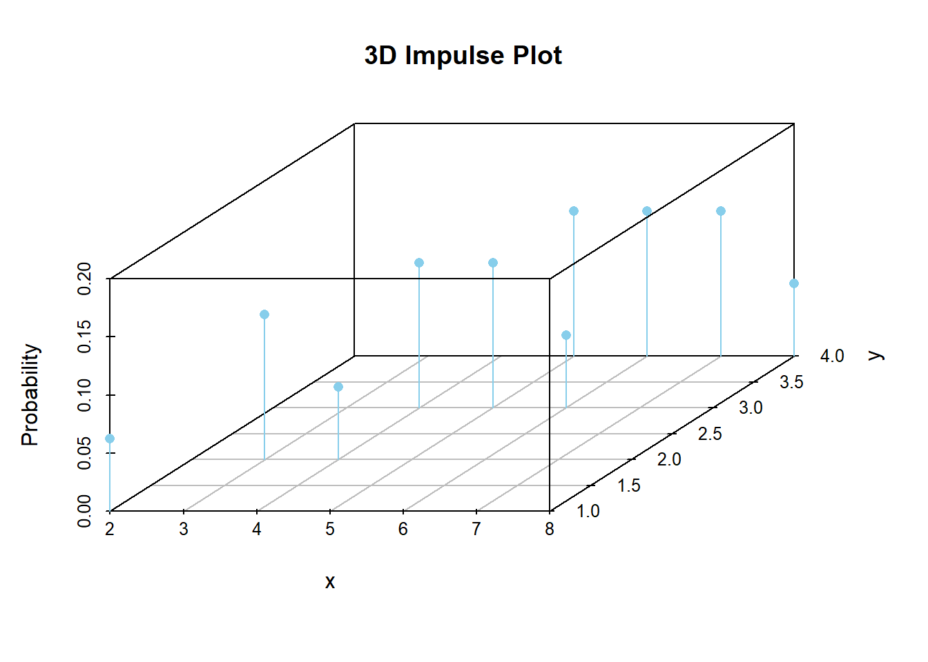
However, 3-d plots can be difficult to visualize. Instead we prefer a tile plot which uses a color scale to represent probability.

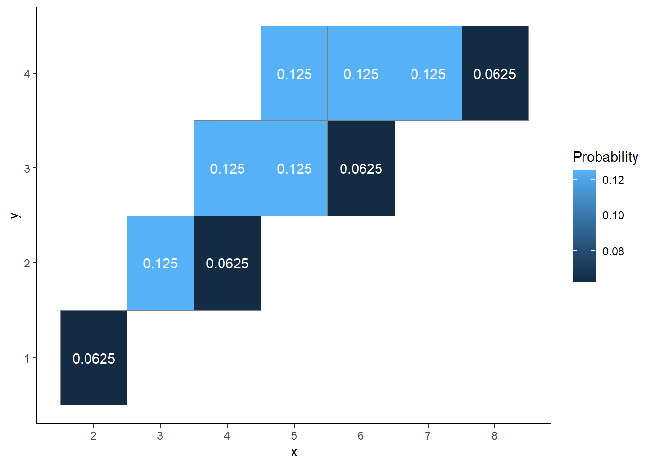
$Tile plot representation of the joint distribution of $X$ and $Y$, the sum and the larger (or common value if a tie) of two rolls of a fair four-sided die. Probability is indicated by the color scale.$

Figure 2.39: Tile plot representation of the joint distribution of $X$ and $Y$, the sum and the larger (or common value if a tie) of two rolls of a fair four-sided die. Probability is indicated by the color scale.

Whichever representation we use, the key is to recognize that the joint distribution of two random variables summarizes the possible pairs of values and their relative likelihoods.

In the context of multiple random variables, the distribution of any one of the random variables is called a marginal distribution. In Example 2.54, we can obtain the marginal distributions of $X$ and $Y$ from the joint distribution by summing rows and columns. Think of adding a total column (for $X$) and a total row (for $Y$) in the “margins” of the table.

It is possible to obtain marginal distributions from a joint distribution. However, in general you cannot recover the joint distribution from the marginal distributions alone. Just because you know the row and column totals doesn’t mean you know all the values of the interior cells in the joint distribution table. The joint distribution reflects the relationship between $X$ and $Y$, while the marginal distributions only reflect how each variable behaves in isolation.

Consider the following two-way table representing the joint distribution of two random variables $X$ and $Y$. You can check that the marginal distributions are the same as in the dice problem. However, clearly the joint distribution of $X$ and $Y$ is not the same as in Table 2.13.

$x$ \ $y$	1	2	3	4
2	0	1/16	0	0
3	1/16	1/16	0	0
4	0	1/16	2/16	0
5	0	0	1/16	3/16
6	0	0	1/16	2/16
7	0	0	0	2/16
8	0	0	1/16	0

In general, marginal distributions alone are not enough to determine a joint distribution. (The exception is when random variables are independent.)

Example 2.55 Continuing the dice rolling example, construct a spinner representing The joint distribution of $X$ and $Y$.

Solution. to Example 2.55.

Show/hide solution

The spinner in Figure 2.40 represents the joint distribution of $X$ and $Y$. For example, the spinner returns the pair $(4, 2)$ with probability 1/16 and the pair $(4, 3)$ with probability 2/16. See Table 2.27 or Table 2.26. Remember, a joint distribution of two random variables is a distribution of pairs on values.

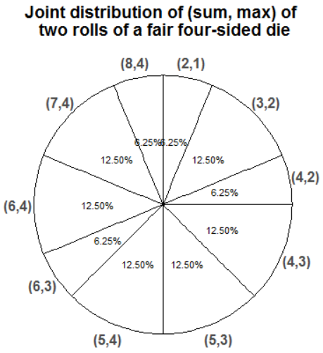
$Spinner representing the joint distribution of $X$ and $Y$, the sum and the larger of two rolls of a fair four-sided die.$

Figure 2.40: Spinner representing the joint distribution of $X$ and $Y$, the sum and the larger of two rolls of a fair four-sided die.

We now have two ways to simulate an $(X, Y)$ pair that has the distribution in Table 2.27.

Simulate two rolls of a fair four sided die. Let $X$ be the sum of the two values and let $Y$ be the larger of the two rolls (or the common value if a tie).
Spin the spinner in Figure 2.40 once and record the resulting $(X, Y)$ pair. (Recall that this spinner returns a pair of values.) Of course, this method requires that the joint distribution of $(X, Y)$ is known.

Below is the Symbulate code for simulating directly from the joint distribution in Table 2.27. Note that the tickets in BoxModel correspond to the possible $(X, Y)$ pairs, which are not equally likely (even though the 16 pairs of rolls are). We specify the probability of each ticket by using the probs option. To generate a single $(X, Y)$ pair — like spinning the spinner in Figure 2.40 once — we draw one ticket from the box of pairs; this is why⁸⁴ size = 1.


xy_pairs = [(2, 1), (3, 2), (4, 2), (4, 3), (5, 3), (5, 4), (6, 3), (6, 4), (7, 4), (8, 4)]
pxy = [1/16, 2/16, 1/16, 2/16, 2/16, 2/16, 1/16, 2/16, 2/16, 1/16]

P = BoxModel(xy_pairs, probs = pxy, size = 1)

P.sim(10)

Index	Result
0	(2, 1)
1	(8, 4)
2	(4, 3)
3	(5, 4)
4	(4, 2)
5	(5, 4)
6	(3, 2)
7	(3, 2)
8	(7, 4)
...	...
9	(3, 2)

We can now define random variables $X$ and $Y$. An outcome of P is a pair of values. Recall that a Symbulate RV is always defined in terms of a probability space and a function RV(probspace, function). The default function is the identity: $g(\omega) = \omega$. Therefore, RV(P) would just correspond to the pair of values generated by P. The sum $X$ corresponds to the first coordinate in the pair and the max $Y$ corresponds to the second. We can define these random variables in Symbulate by “unpacking” the pair as in the following⁸⁵

X, Y = RV(P)

Then we can simulate many $(X, Y)$ pairs and summarize as we have done previously.

(RV(P) & X & Y).sim(10)

Index	Result
0	((8, 4), 8, 4)
1	((6, 4), 6, 4)
2	((4, 3), 4, 3)
3	((4, 3), 4, 3)
4	((7, 4), 7, 4)
5	((8, 4), 8, 4)
6	((6, 3), 6, 3)
7	((7, 4), 7, 4)
8	((5, 3), 5, 3)
...	...
9	((6, 3), 6, 3)

(X & Y).sim(10000).plot('tile')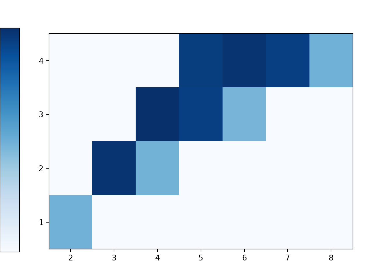

Example 2.56 Donny Don’t says “Now I see why we need the spinner in Figure 2.40 to simulate $(X, Y)$ pairs. So then forget the marginal spinners in Figure 2.30 and Figure 2.31. If I want to simulate $X$ values, I could just spin the joint distribution spinner in Figure 2.40 and ignore the $Y$ values.” Is Donny’s method correct? If not, can you help him see why not?

Solution. to Example 2.56

Show/hide solution

Donny is correct! The joint distribution spinner in Figure 2.40 correctly produces $(X, Y)$ pairs according to the joint distribution in Table 2.27. Ignoring the $Y$ values is like “summing the rows” and only worrying about what happens in total for $X$. For example, in the long run, 1/16 of spins will generate (4, 2) and 2/16 of spins will generate (4, 3), so ignoring the $y$ values, 3/16 of spins will return an $x$ value of 4. From the joint distribution you can always find the marginal distributions (e.g., by finding row and column totals).

Now, Donny’s method does work, but it does require more work than necessary. If we really only needed to simulate $X$ values, we only need the distribution of $X$ and not the joint distribution of $X$ and $Y$, so you could use the $X$ spinner in Figure 2.30. But if we wanted to study anything about the relationship between $X$ and $Y$ then we would need the joint distribution spinner.

2.11.2 Joint distributions of two continuous random variables

Consider the meeting problem where Regina ($R$) and Cady ($Y$) are each assumed to arrive according to a Normal(30, 10) distribution, independently of each other. We can approximate the joint distribution of $R$ and $Y$ by simulating many $(R, Y)$ pairs.

R, Y = RV(Normal(30, 10) ** 2)

r_and_y = (R & Y).sim(10000)

r_and_y.plot()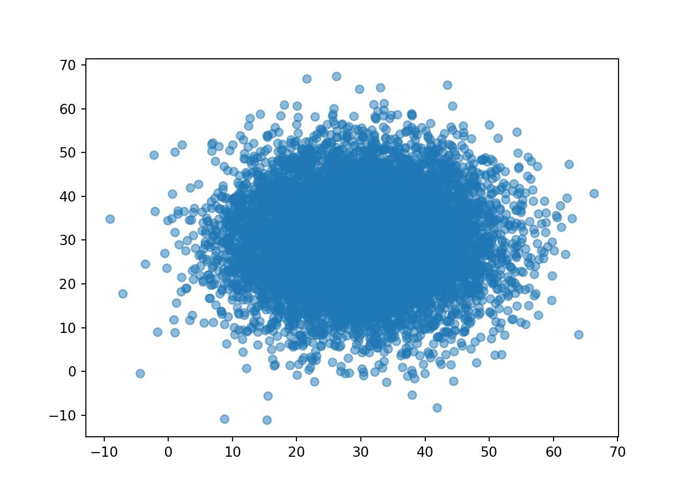

Unfortunately, a scatterplot does not provide the best visual of the relative frequencies of different regions of $(R, Y)$ pairs. Instead, we can summarize the simulated values in a 2-dimensional histogram which chops the region of possible values into rectangular “bins” and displays the relative frequency of pairs falling in each bin with a color scale.

r_and_y.plot('hist')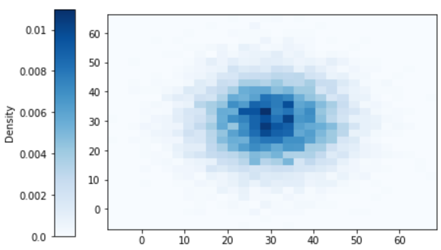

We see that pairs near (30, 30) occur more frequently than those near the “corners”.

A 2-d histogram is a flat representation of a 3-d plot; each bin would have a bar with a density height chosen so that the volume of the bar is its relative frequency. If we simulate more and more values, and make the bins smaller and smaller, a smooth “density” surface would emerge.

Three-dimensional plots are hard to visualize so tend to use heat maps or contour plots to represent joint distributions of two continuous random variables.

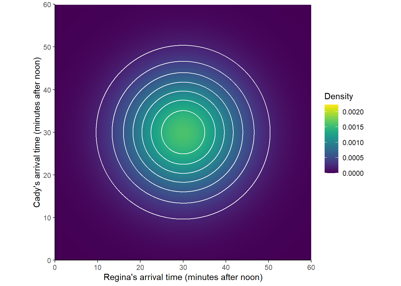
The marginal distribution of a single continuous random variable can be described by a probability density function, for which areas under the curve determine probabilities. Likewise, the joint distribution of two continuous random variables can be described by a probability density function, for which volumes under the surface determine probabilities. The “density” height is whatever it needs to be so that volumes under the surface represent appropriate probabilities.

Continuing the meeint problem, let $T=\min(R, Y)$ be the time at which the first person arrives, and let $W=|R-Y|$ be the amount of time the first person to arrive has to wait for the second person to arrive. We can use simulation to investigate the joint distribution of $T$ and $W$. We see that there appears to be a negative association between $T$ and $W$: larger values of $T$ tend to occur with smaller values of $W$. We can measure the strength of this association with the correlation, which we will investigate further in the next section.


W = abs(R - Y)

T = (R & Y).apply(min)

t_and_w = (T & W).sim(10000)

t_and_w.plot('hist')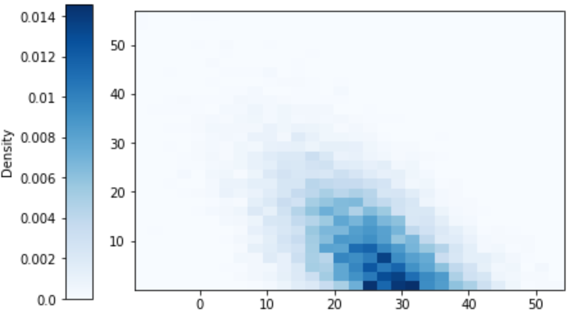


t_and_w.corr()

## -0.5271192883725928

We can obtain marginal distributions from a joint distribution by “stacking”/“collapsing”/“aggregating” out the other variable. Imagine a joint histogram with blocks of different heights for each $(x, y)$ bin. To find the marginal distribution of $X$ for a particular $x$ interval stack all the bars for the $(x, y)$ bins — same $x$ but different $y$ — on top of each other, “collapsing out” the $y$’s.

t_and_w.plot(['hist', 'marginal'])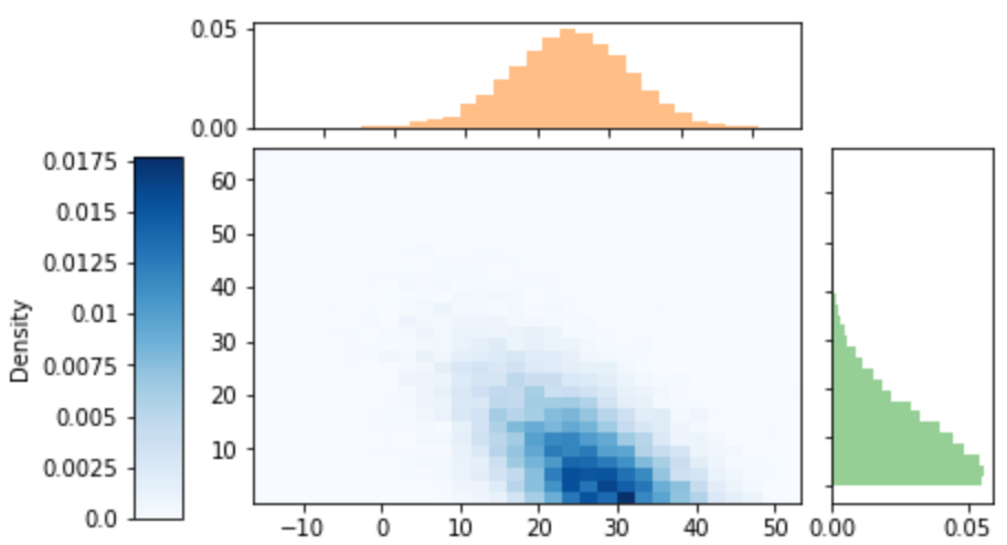

We mostly focus on the case of two random variables, but analogous definitions and concepts apply for more than two (though the notation can get a bit messier).↩︎
By default size = 1, so we could have omitted it, but we include it for emphasis. Drawing 1 ticket from this box model returns an $(X, Y)$ pair.↩︎
Since P returns pairs of outcomes, Z = RV(P) is a random vector. Components of a vector can be indexed with brackets []; e.g., the first component is Z[0] and the second is Z[1]. (Remember: Python uses zero-based indexing.) So the “unpacked” code is an equivalent but simpler version of Z = RV(P); X = Z[0]; Y = Z[1].↩︎

\(x\) \ \(y\)	1	2	3	4
2	1/16	0	0	0
3	0	2/16	0	0
4	0	1/16	2/16	0
5	0	0	2/16	2/16
6	0	0	1/16	2/16
7	0	0	0	2/16
8	0	0	0	1/16