2.1 Sample space of outcomes

Probability models can be applied to any situation in which there are multiple potential outcomes and there is uncertainty about which outcome will occur. Due to the wide variety of types of random phenomena, an outcome can be virtually anything:

the result of a coin flip
the results of a sequence of coin flips
a shuffle of a deck of cards
the weather conditions tomorrow in your city
the path of a particular Atlantic hurricane
the daily closing price of a certain stock over the next 30 days
the result of a diagnostic medical test
a sample of car insurance polices
the customers arriving at a store
the result of an election
the next World Series champion
a play in a basketball game

And on and on. In particular, an outcome does not have to be a number.

Before the random phenomenon occurs it is unknown which outcome will be the result. When the phenomenon takes place, a particular outcome is observed. The first step in defining a probability model for a random phenomenon is to identify the possible outcomes.

Definition 2.1 The sample space, denoted²⁰ $\Omega$ (the uppercase Greek letter “omega”), is the set of all possible outcomes of a random phenomenon. An outcome, denoted $\omega$ (the lowercase Greek letter “omega”), is an element of the sample space: $\omega\in\Omega$.

Mathematically, the sample space $\Omega$ is a set containing all possible outcomes, while an individual outcome $\omega$ is a point or element in $\Omega$. The symbol $\omega$ denotes a generic outcome, much like the symbol $u$ in $\sqrt{u}$ denotes a generic input to the square root function.

The simplest random phenomena have just two distinct outcomes, in which case the sample space is just a set with two elements, e.g. $\Omega=\{\text{no}, \text{yes}\}$, $\Omega=\{\text{off}, \text{on}\}$, $\Omega=\{0, 1\}$, $\Omega=\{-1, 1\}$. For example, the sample space for a single coin flip could be $\Omega = \{H, T\}$. If the coin lands on heads, we observe the outcome $\omega = H$; if tails we observe $\omega=T$.

A random phenomenon is modeled by a single sample space, upon which all objects are defined. These objects, which we will encounter later, include events and random variables. Whenever possible, a sample space outcome should be defined to provide the maximum amount of information about the outcome of random phenomenon.

In the following examples we will describe the sample space by listing all possible outcomes. However, constructing a list of all possible outcomes is rarely done in practice. We do so here only to provide some concrete examples of sample spaces. While a random phenomenon always has a corresponding sample space, in most situations the sample space of outcomes is at best only vaguely specified and can not be feasibly enumerated.

Example 2.1 Roll a four-sided die²¹ twice, and record the result of each roll in sequence as an ordered pair. For example, the outcome $(3, 1)$ represents a 3 on the first roll and a 1 on the second; this is not the same outcome as $(1, 3)$.

Identify the sample space.
We might be interested in the sum of the two rolls. Explain why it is still advantageous to define the sample space as in the previous part, rather than as $\Omega=\{2, \ldots, 8\}$.

Solution. to Example 2.1

Show/hide solution

We simply enumerate all the possible outcomes: first roll is a 1 and second roll is a 1, first roll is a 1 and second roll is a 2, etc. The sample space consists of 16 possible ordered pairs of rolls \[\begin{align*} \Omega & = \{(1, 1), (1, 2), (1, 3), (1, 4),\\ & \qquad (2, 1), (2, 2), (2, 3), (2, 4),\\ & \qquad (3, 1), (3, 2), (3, 3), (3, 4),\\ & \qquad (4, 1), (4, 2), (4, 3), (4, 4)\} \end{align*}\] Any element of this set is a possible outcome $\omega$. For example, the outcome $\omega = (4, 2)$ occurs when the first roll is a 4 and the second roll is a 2. The notation above makes it clear that the sample space is a set. But it is often helpful to conceptualize or visualize the sample space as a list or table as in Table 2.1.
Yes, we might be interested in the sum of the two dice. But we might also be interested in other things, like the larger of the two rolls, or if at least one 3 was rolled, or the result of the first roll. Knowing just the sum of the rolls does not provide as much information about the outcome of the random phenomenon as the sequence of individual rolls does.

Table 2.1: Table representing the sample space of two rolls of a four-sided die. Each row represents an outcome.
First roll	Second roll
1	1
1	2
1	3
1	4
2	1
2	2
2	3
2	4
3	1
3	2
3	3
3	4
4	1
4	2
4	3
4	4

In the previous example, there was a single sample space whose outcomes represented the result of the pair of rolls. In particular, there was not a separate sample space for each of the individual rolls. We could have written the sample space as the Cartesian product $\Omega = \{1, 2, 3, 4\} \times\{1, 2, 3, 4\}$, where the first $\{1, 2, 3, 4\}$ set in the product represents the result of the first roll (and similarly for the second). But this Cartesian product still represents a single set of ordered pairs, and it is that single set which is the sample space corresponding to outcomes of the pair of rolls.

Example 2.2 Consider the outcome of a sequence of 4 flips of a coin.

Identify an appropriate sample space.
We might be interested in the number of heads flipped. Explain why it is still advantageous to define the sample space as in the previous part, rather than as $\Omega=\{0, 1, 2, 3, 4\}$.

Solution. to Example 2.2

Show/hide solution

We can record the outcome as an ordered sequence representing the results of the four flips. For example, HTHT means heads on the first and third flips and tails on the second and fourth flips; this is not the same outcome as HHTT or THTH. (We could also write (H, T, H, T) but the HTHT notation is simpler.) The sample space is the following set composed of 16 distinct outcomes \[\begin{align*} \Omega & = \{HHHH, HHHT, HHTH, HTHH, THHH, HHTT, HTHT, HTTH,\\ & \qquad THHT, THTH, TTHH, HTTT, THTT, TTHT, TTTH, TTTT\} \end{align*}\] Again, it is helpful to conceptualize and visualize the sample space as a list or a table (which we will do later when we encounter this scenario again).
Yes, we might be interested in the number of heads flipped, but we might also be interested in other things, such as whether the first flip was heads, the length of the longest streak of heads in a row, or the proportion of flips following H that resulted in H. Knowing just the number of heads flipped does not provide as much information about the outcome of the random phenomenon as the sequence of individual flips does.

We reiterate what we said after Example 2.1. In the previous example, there was a single sample space whose outcomes were sequences of coin flips. In particular, there was not a separate sample space for each of the individual flips. We could have written the sample space as the Cartesian product $\Omega = \{H, T\}\times \{H, T\}\times \{H, T\}\times \{H, T\} = \{H, T\}^4$. But this Cartesian product represents a single set whose elements are sequences of 4 flips, and it is this single set which is the sample space.

We’ll present a few more concrete examples where we list all the outcomes in the sample space. However, keep in mind that enumerating the sample space is rarely done in practice.

Example 2.3 (Matching problem) Rocks labeled 1, 2, 3, 4, are placed at random in spots labeled 1, 2, 3, 4, with spot 1 the correct spot for rock 1, etc. We might be interested in things like whether all the rocks are put back in the correct spot, or none are, or if rock 1 is put back in the correct spot. Identify an appropriate sample space.

Solution. to Example 2.3

Show/hide solution

We can consider each outcome to be a particular placement of rocks in the spots. For example, the outcome 3214 (or $(3, 2, 1, 4)$) represents that rock 3 is placed in spot 1, rock 2 in spot 2, rock 1 in spot 3, and rock 4 in spot 4. (We say that an outcome is a permutation (or reordering) of the numbers 1, 2, 3, 4.) So the sample space consists of the following 24 outcomes²².

\[\begin{align*} \Omega & = \{1234, 1243, 1324, 1342, 1423, 1432 \\ & \qquad 2134, 2143, 2314, 2341, 2413, 2431 \\ & \qquad 3124, 3142, 3214, 3241, 3412, 3421 \\ & \qquad 4123, 4132, 4213, 4231, 4312, 4321\} \end{align*}\]

Recording outcomes in this way provides more information than if we had chosen the sample space to correspond to, for example, the number of rocks that were placed in the correct spot.

Example 2.4 (Collector problem) The latest series of collectible Lego Minifigures contains 3 different Minifigures. Each package contains a single unknown Minifigure. We buy packages one at a time. We might be interested in things like how many packages we need to buy to complete the collection, or how many packages we need to buy to complete 5 collections (say one collection for each of 5 kids), or which Minifigure we have the most of.

Label the different Minifigures 1, 2, and 3. Identify an appropriate sample space. Is it possible to identify a sample space in which all outcomes have the same “length”?

Solution. to Example 2.4

Show/hide solution

An outcome could represent the sequence of Minifigures we obtain in order. For example, (2, 3, 3, 2, 2, 2, 3, 1) represents figure 2 in the first package, figure 3 in the second and third packages, figure 2 in the fourth, and so on, completing a collection with figure 1 in the eighth package. Outcomes recorded in this way can have different lengths if we only record the packages we buy until we complete a collection; for example (2, 3, 1) versus (2, 3, 3, 1) versus (2, 3, 3, 2, 1). However, it is often convenient for sample space outcomes to have the same length, as in the previous examples (two die rolls, four coin flips, four rocks in spots).

We can define outcomes with the same “length” if we assume the process continues indefinitely, that is, if we continue to buy packages even after we complete a set. Now an outcome is an infinite sequence, with each component of the sequence taking a value of 1, 2, or 3; for example, (2, 3, 3, 2, 2, 2, 3, 1, 2, 1, 1, 3, $\ldots$). Thus the sample space is the set of all infinite sequences whose components take values in $\{1, 2, 3\}$, which can be written as $\Omega=\{1, 2, 3\}^\infty$. Outcomes of this sample space all have the same “length” (infinite). Moreover, this sample space allows for a broader range of questions to be investigated. For example, we might be interested in the number of packages needed to obtain 5 complete collections (which might be relevant if you have 5 kids and they all want their own collection).

Example 2.5 Many statistical applications involve random sampling. For example, polling organizations often select random samples of Americans. Typically the selection involves random digit dialing: a sample of say 1000 phone numbers are randomly selected from some large bank (hundreds of millions) of phone numbers; this is the population²³. An outcome would consist of the 1000 phone numbers selected; this is the sample.

As an extraordinarily unrealistic, oversimplified, but concrete example, suppose the bank only contains 5 phone numbers, labeled {1, 2, 3, 4, 5}, from which 3 are selected. Describe an appropriate sample space. Note: the order in which the numbers are selected does not matter; we only care which numbers are selected.

Solution. to Example 2.5

Show/hide solution

An outcome consists of a subset of size 3 from the set $\{1, 2, 3, 4, 5\}$, representing the list of the 3 phone numbers selected. For example, outcome $\{1, 4, 5\}$ occurs if phone numbers 1, 4, and 5 are selected. There are 10 distinct outcomes \[ \Omega = \{\{1, 2, 3\}, \{1, 2, 4\}, \{1, 2, 5\}, \{1, 3, 4\}, \{1, 3, 5\},\\ \qquad\quad \{1, 4, 5\}, \{2, 3, 4\},\{2, 3, 5\},\{2, 4, 5\},\{3, 4, 5\}\} \] Note that the sample space is a set whose elements are sets. Also note the difference between $\{1, 2, 3\}$ and $(1, 2, 3)$ — $\{1, 2, 3\}$ represents an unordered set; $(1, 2, 3)$ represents an ordered sequence. There is only one set containing the elements 1, 2, and 3, the set $\{1, 2, 3\}$, but there are six different ordered sequences containing the values 1, 2, and 3: $(1, 2, 3), (1, 3, 2), (2, 1, 3), (2, 3, 1), (3, 1, 2), (3, 2, 1)$.

In a more realistic setting, the population would consist of hundreds of millions of phone numbers, and the sample space²⁴ would be composed of all possible subsets (samples) of 1000 phone numbers. Even if the order in which the numbers are selected is irrelevant, the sample space is enormous and could never be feasibly enumerated as in this oversimplified example. But the idea is the same: an outcome consists of a subset of numbers, and the sample space is a collection of possible subsets. (That is, the sample space is a set of sets.)

Example 2.6 (Meeting problem) Regina and Cady plan to meet for lunch between noon and 1 but they are not sure of their arrival times. We might be interested in questions involving whether they arrive within 15 minutes of one another, who arrives first, or how long the first person to arrive needs to wait for the second.

Describe an appropriate sample space. Note: rather than dealing with clock time, it is helpful to represent noon as time 0 and measure time as fraction of the hour after noon, so that times take values in the continuous interval [0, 1]. For example, 12:15 corresponds to a time of 0.25, 12:30 to 0.5, 12:42 to 0.7.

Solution. to Example 2.6

Show/hide solution

An outcome is a pair of values $\omega = (\omega_1, \omega_2)$ corresponding to the arrival times of (Regina, Cady). For example, the outcome (0.5, 0.7) represents Regina arriving at time 0.5 (12:30) and Cady at time 0.7 (12:42), while (0.7, 0) represents Regina arriving at time 0.7 (12:42) and Cady at time 0 (noon). The sample space is $\Omega = [0,1]\times [0,1]=[0,1]^2$, the Cartesian product $\{(\omega_1, \omega_2): \omega_1 \in [0, 1], \omega_2 \in [0, 1]\}$, the set of ordered pairs whose components take values in $[0, 1]$. This sample space is an uncountable set, and it is impossible to enumerate outcomes like in the previous examples. (The sample space of infinite sequences in Example 2.4 is also an uncountable set.) We can visualize the sample space as the set of points within the blue square in Figure 2.1.

$The square represents the sample space $\Omega=[0,1]\times[0,1]$ in Example 2.6. Each point within the blue square is a pair of values $\omega = (\omega_1, \omega_2)$ corresponding to the arrival times of (Regina, Cady).$

Figure 2.1: The square represents the sample space $\Omega=[0,1]\times[0,1]$ in Example 2.6. Each point within the blue square is a pair of values $\omega = (\omega_1, \omega_2)$ corresponding to the arrival times of (Regina, Cady).

A value in $[0, 1]$ can be visualized with a circular spinner like the one in Figure 2.2 which returns values between 0 and 1. Such a spinner can be thought of as a continuous analog of a die roll. Imagine a needle anchored at the center of the circle which is spun and eventually lands pointing at a number on the outside of the circle (like a spinner in a kids game). The values in the picture are rounded to two decimal places, but consider an idealized model where the spinner is infinitely precise and the needle infinitely fine so that any real number between 0 and 1 is a possible outcome. Under certain assumptions in the meeting time problem, we can think of Regina and Cady each spinning the spinner, with the results of the pair of spins representing the outcome $\omega$. (But under other assumptions the spinner in Figure 2.2 might not be appropriate, if for example, Regina is more likely to arrive later in the hour and Cady is more likely to arrive earlier in the hour.)

Figure 2.2: A Uniform(0, 1) spinner. The values in the picture are rounded to two decimal places, but in the idealized model the spinner is infinitely precise so that any real number between 0 and 1 is a possible outcome.

In the previous example, outcomes were measured on a continuous scale; any real number between 0 and 1 was a possible arrival time (or a possible result of a spin). In practice we might round the arrival time to the nearest minute or second, but in principle and with infinite precision any real number in the continuous interval $[0, 1]$ is possible.

Furthermore, even in situations where outcomes are inherently discrete, it is often more convenient to model them as continuous. For example, if an outcome represents the annual salary in dollars of a randomly selected U.S. household, it would be more convenient to model the sample space as the continuous interval²⁵ $[0, \infty)$ rather than $\{0, 1, 2, \ldots\}$ or $\{0, 0.01, 0.02, \ldots\}$.

Example 2.7 Select a U.S. high school student and record the student’s SAT Math and Reading scores. Identify an appropriate sample space.

Solution. to Example 2.7

Show/hide solution

An outcome will be an ordered pair representing (Math, Reading) score. Technically, possible scores are 200 through 800 in increments of 10. So we could consider the sample space to be $\{200, 210, 220, \ldots, 790, 800\}\times \{200, 210, 220, \ldots, 790, 800\}$.

However, we could also model scores on a continuous scale, taking any value in the interval from 200 to 800. In this case, the sample space would be $\Omega = [200, 800] \times [200, 800]$. This sample space could be represented in a square like the one in Figure 2.1, but with Math score on the horizonal axis, Reading score on the vertical, and axis limits of $[200, 800]$ instead of $[0, 1]$. A continuous specification of a sample space is often more convenient mathematically than a discrete one.

In the previous examples, the sample space could be defined rather explicitly, either by direct enumeration or using set notation (like a Cartesian product). However, explicitly defining a sample space in a compact way is often not possible, as in the following example.

Example 2.8 Customers enter a deli and take a number to mark their place in line. When the deli opens the counter starts 0; the first customer to arrive takes number 1, the second 2, etc. We record the counter over time, continuously, as it changes as customers arrive. Time is measured in minutes after the deli opens (time 0). How might you define an appropriate sample space?

Solution. to Example 2.8

Show/hide solution

A sample space outcome could be represented as a path of the value of the counter over time; a few such paths are illustrated in Figure 2.3. Notice the stairstep feature: a customer arrives and takes a number then the counter stays on that number for some time (the flat spots) until another customer arrives and the counter increases by one (the jumps). In other words, an outcome is a nondecreasing function mapping the time interval $[0, \infty)$ to nonnegative integers $\{0, 1, 2, \ldots\}$, that only jumps by one unit at a time. The sample space consists of all possible functions of this form.

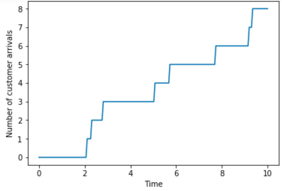
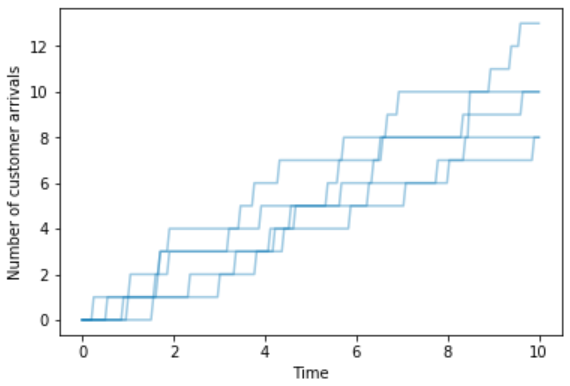
Sample space outcomes for Example 2.8. Left: a single sample path of the number of customer arrivals over time. Right: several possible paths.

Figure 2.3: Sample space outcomes for Example 2.8. Left: a single sample path of the number of customer arrivals over time. Right: several possible paths.

Any random phenomenon has a corresponding sample space but in some situations explicitly defining a outcome is not feasible. For example, consider a single play in a basketball game. The SportsVU system uses cameras in arenas to record NBA games. The outcome of a single play might look like this video.

In order to describe such an outcome, we need to specify (among other things): the location of each player and the ball, the passer and receiver of each pass, the defensive assignments, the location and shooter of each shot attempt and its result, and how it all evolves over time. Representing all of this information in a compact way to define an outcome is virtually impossible. Regardless, the sample space is still there in the background, whether we specify it or not. Without a sample space representing what is possible, we would not be able to assess the relative likelihood of, say, a play resulting in a made three point field goal.

2.1.1 Summary

The sample space is the set of all possible outcomes of a random phenomenon.
Outcomes can take a wide variety of forms. In particular, outcomes do not need to be numbers.
Whenever possible, a sample space outcome should be defined to provide the maximum amount of information about the outcome of random phenomenon.

In practice we rarely enumerate the sample space as we did for some of the examples in this section. Nonetheless, there is always some underlying sample space corresponding to all possible outcomes of the random phenomenon. Even though the sample space often plays a background role, it is important to first consider what is possible before determining what is probable. The sample space essentially defines the denominator in probability calculations. Considering the sample space can help distinguish between “what is the probability this happens to me?” and “what is the probability this happens to someone somewhere sometime?” (as discussed in Section 1.5.)

2.1.2 Exercises

In Example 2.4, suppose we only buy 3 packages. Identify a sample space to represent the results of the 3 packages. (Hint: there should be 27 outcomes.)
Randomly select a baseball game and record the total number of runs scored and the length of the game. Identify an appropriate sample space.
Two players, A and B, play a single game of rock, paper, scissors (RPS). What specification of an outcome provides the most possible information about the game? Specify the corresponding sample space.

There is no one set of universally agreed on notation, but $\Omega$ is commonly used to represent a sample space. It is also common practice to use uppercase and lowercase letters to denote different objects, like $\Omega$ versus $\omega$.↩︎
Why four-sided? Simply to make the number of possibilities a little more manageable (e.g., for in-class simulation activities). Rolling a four-sided die twice yields 16 possible pairs, while rolling a six-sided die yields 36 possible pairs.↩︎
There are 4 rocks that could potentially go in spot 1, then 3 rocks that could potentially go in spot 2, 2 to spot 3, and 1 left for spot 4. This results in $4\times3\times2\times1=4! = 24$ possible outcomes. We will see more counting rules later.↩︎
Technically, the bank of phone numbers is the sampling frame while the population might be all Americans. The population and the sampling frame need not be the same.↩︎
We are unaware of the origin or history of the term “sample space”, but in the context of random sampling from a population, the sample space can be thought of as the space of possible samples.↩︎
We could also try $[0, m]$ where $m$ is some large dollar amount providing an upper bound on the maximum possible salary. But we would need to be sure that $m$ is large enough so that all possible outcomes are in the sample space $[0, m]$. Without knowing this bound in advance, it is convenient to just choose the unbounded interval $[0, \infty)$. There is really no harm in making the sample space bigger than it needs to be, but you can run into problems if you make it too small.↩︎