4.9 Transformations of multiple random variables

Earlier in this chapter we studied the joint distribution of the sum and max of two fair-four sided dice rolls. Now we consider a continuous analog. Instead of rolling a die which is equally likely to take the values 1, 2, 3, 4, we spin a Uniform(1, 4) spinner that lands uniformly in the continuous interval $[1, 4]$. Let $\textrm{P}$ be the probability space corresponding to two spins of the Uniform(1, 4) spinner, and let $X$ be the sum of the two spins, and $Y$ the larger spin (or the common value if a tie). We saw that in Section 4.1, we could model two rolls of a fair-four sided die using DiscreteUniform(1, 4) ** 2. Similarly, we can model two spins of the Uniform(1, 4) spinner with Uniform(1, 4) ** 2.

We start by looking at the joint distribution of the two spins, $(U_1, U_2)$, which take values in $[1, 4]\times[1, 4]$.


P = Uniform(1, 4) ** 2
U1, U2 = RV(P)

u1u2 = (U1 & U2).sim(100)


u1u2.plot()
plt.show()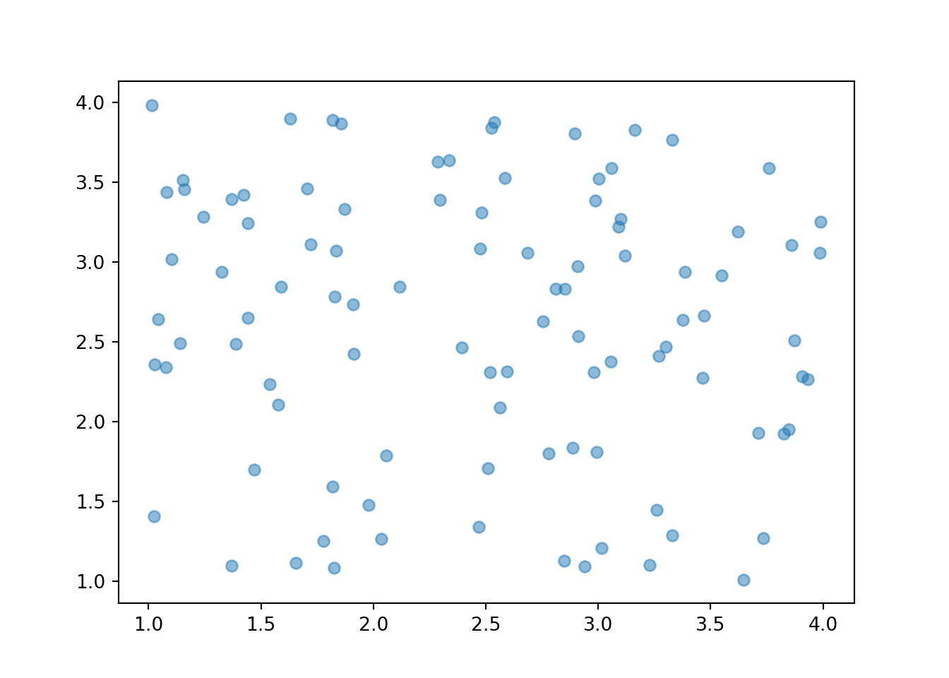

We see that the $(U_1, U_2)$ pairs are roughly “evenly spread” throughout $[1, 4]\times [1, 4]$. The scatterplot displays each individual pair. We can summarize the distribution of many pairs with a two-dimensional histogram. To construct the histogram, the space of values $[1, 4]\times[1, 4]$ is chopped into rectangular bins and the relative frequency of pairs which fall within each bin is computed. In a histogram of a single variable, area represents relative frequency; in a histogram of two variables, volume represents relative frequency, with the height of each rectangular bin on a “density” scale represented by its color intensity.


(U1 & U2).sim(10000).plot('hist')

## Error in py_call_impl(callable, dots$args, dots$keywords): ValueError: invalid literal for int() with base 10: ''

plt.show()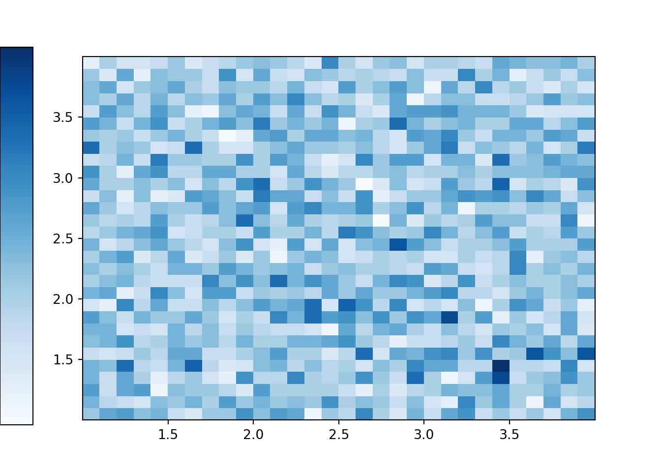

Now we let $X$ be the sum and $Y$ the max of the two spins⁸⁶. First consider the possible values of $(X, Y)$. Marginally, $X$ takes values in $[2, 8]$ and $Y$ takes values in $[1, 4]$. However, not every value in $[2, 8]\times [1, 4]$ is possible. Before proceeding, sketch a picture representing the possible values of $(X, Y)$ pairs.

We must have $Y \ge 0.5 X$, or equivalently, $X \le 2Y$. For example, if $X=4$ then $Y$ must be at least 2, because if the larger of the two spins were less than 2, then both spins must be less than 2, and the sum must be less than 4.
We must have $Y \le X - 1$, or equivalently, $X \ge Y + 1$. For example, if $Y=3$, then one of the spins is 3 and the other one is at least 1, so the sum must be at least 4.

Therefore, the possible values of $(X, Y)$ lie in the set \[ \{(x, y): 2\le x\le 8, 1 \le y\le 4, 0.5x \le y \le x-1\} \] which can also be written as $\{(x, y): 2\le x \le 8, 0.5 x\le y \le \min(4, x-1)\}$. This set is represented by the triangular region in the plots below.


P = Uniform(1, 4) ** 2

U = RV(P)
X = RV(P, sum)
Y = RV(P, max)

(U & X & Y).sim(100)

Index	Result
0	((3.712073389186292, 1.2440329977043403), 4.956106386890632, 3.712073389186292)
1	((3.0480154603437337, 2.7849913857530186), 5.833006846096753, 3.0480154603437337)
2	((1.5877606021241109, 3.7189358122967953), 5.306696414420906, 3.7189358122967953)
3	((3.260914240311907, 3.6927568830355373), 6.953671123347444, 3.6927568830355373)
4	((2.1961354969055566, 3.592788519065761), 5.788924015971318, 3.592788519065761)
5	((1.506590237044053, 2.1624606368441768), 3.6690508738882297, 2.1624606368441768)
6	((3.6000334429380585, 2.451351119119929), 6.051384562057987, 3.6000334429380585)
7	((2.8769906498460878, 3.683066482920905), 6.5600571327669925, 3.683066482920905)
8	((2.2683969414576977, 3.9089039001228474), 6.177300841580545, 3.9089039001228474)
...	...
99	((3.616509213650626, 1.066731751963216), 4.683240965613842, 3.616509213650626)


(X & Y).sim(100).plot()
plt.show()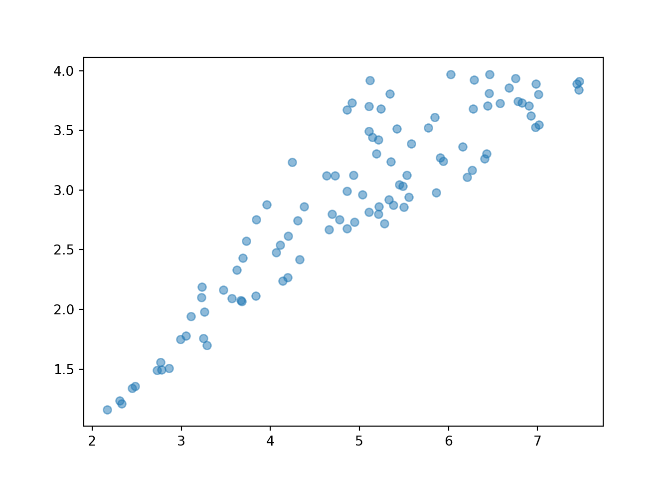



(X & Y).sim(10000).plot('hist')

## Error in py_call_impl(callable, dots$args, dots$keywords): ValueError: invalid literal for int() with base 10: ''

plt.show()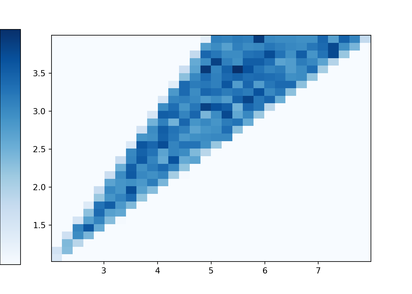

Compare the joint histogram above to the tile plot in Section 3.4.7. In the dice rolling situation there are basically two cases. Each $(X, Y)$ pair that correspond to a tie — that is each $(X, Y)$ pair with $X = 2Y$ — has probability 1/16. Each of the other possible $(X, Y)$ pairs has probability 2/16.

Back to the continuous analog, the histogram shows that $(X, Y)$ pairs are roughly uniformly distributed within the triangular region of possible values. Consider a single $(X, Y)$ pair, say (0.8, 0.5). There are two outcomes — that is, pairs of spins — for which $X=0.8, Y=0.5$, namely (0.5, 0.3) and (0.3, 0.5). Like (0.8, 0.5), most of the possible $(X, Y)$ values correspond to exactly two outcomes. The only ones that do not are the values with $Y = 0.5X$ that lie along the south/east border of the triangular region. The pairs $(X, 0.5X)$ only correspond to exactly one outcome. For example, the only outcome corresponding to (6, 3) is the $(U_1, U_2)$ pair (3, 3); that is, the only way to have $X=6$ and $Y=3$ is to spin 3 on both spins. In general, the event $\{Y = 0.5X\}$ is the same as the event that both spins are exactly the same, $\{U_1=U_2\}$. However, as discussed in Section 2.4.5, the probability that $U_1=U_2$ exactly is 0. Therefore, we don’t really need to worry about the ties as we did in the discrete case. Excluding ties, roughly, each pair in the triangular region of possible $(X, Y)$ pairs corresponds to exactly two outcomes (pairs of spins), and since the outcomes are uniformly distributed (over $[1, 4]\times[1, 4]$) then the $(X, Y)$ pairs are also uniformly distributed (over the triangular region of possible values).

The plot below represents the joint distribution of $(X, Y)$. This is really a three-dimensional plot. The base is the triangular region which represents the possible $(X, Y)$ pairs. There is a surface floating above this region which represents the density at each point. For a single variable, the density is a smooth curve approximating the idealized shape of the histogram. Likewise, for two variables, the density is a smooth surface approximating the idealized shape of the joint histogram. The height of this surface is depicted in the two-dimensional plot via the color intensity. Since the $(X, Y)$ pairs are uniformly distributed over their range of possible values, the height of the surface and hence the color intensity is constant over the range of possible values, and the height is 0 (white) for impossible $(X, Y)$ pairs. Careful: this plot is not the same as the ones in Section 2.4.5. Those plots were just depicting events, and the color was just used to shade the region of interest. The plot below is depicting a joint distribution, and the color represents the height of the density surface at each $(X, Y)$ pair; white areas correspond to a height of 0.

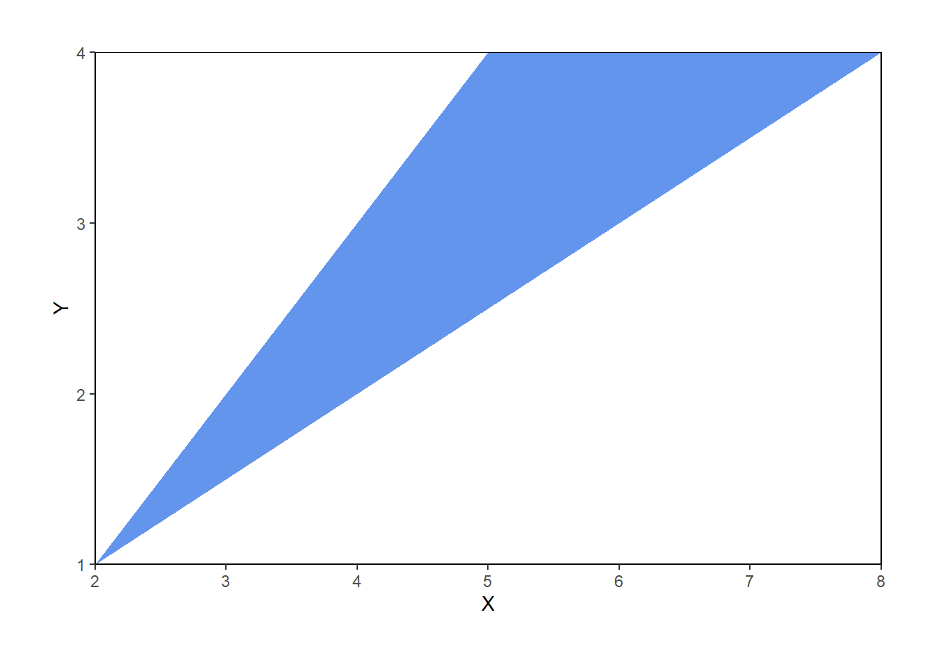
$Joint distribution of $X$ (sum) and $Y$ (max) of two spins of the Uniform(1, 4) spinner. The triangular region represents the possible values of $(X, Y)$ the height of the density surface is constant over this region and 0 outside of the region.$

Figure 4.9: Joint distribution of $X$ (sum) and $Y$ (max) of two spins of the Uniform(1, 4) spinner. The triangular region represents the possible values of $(X, Y)$ the height of the density surface is constant over this region and 0 outside of the region.

We now consider the marginal distributions of $X$ and $Y$. Before proceeding, try to sketch the marginal distributions.

Here is a plot showing the joint histogram representing the joint distribution of $(X, Y)$, along with histograms representing each of the marginal distributions.


(X & Y).sim(10000).plot(['hist', 'marginal'])

## Error in py_call_impl(callable, dots$args, dots$keywords): ValueError: invalid literal for int() with base 10: ''

plt.show()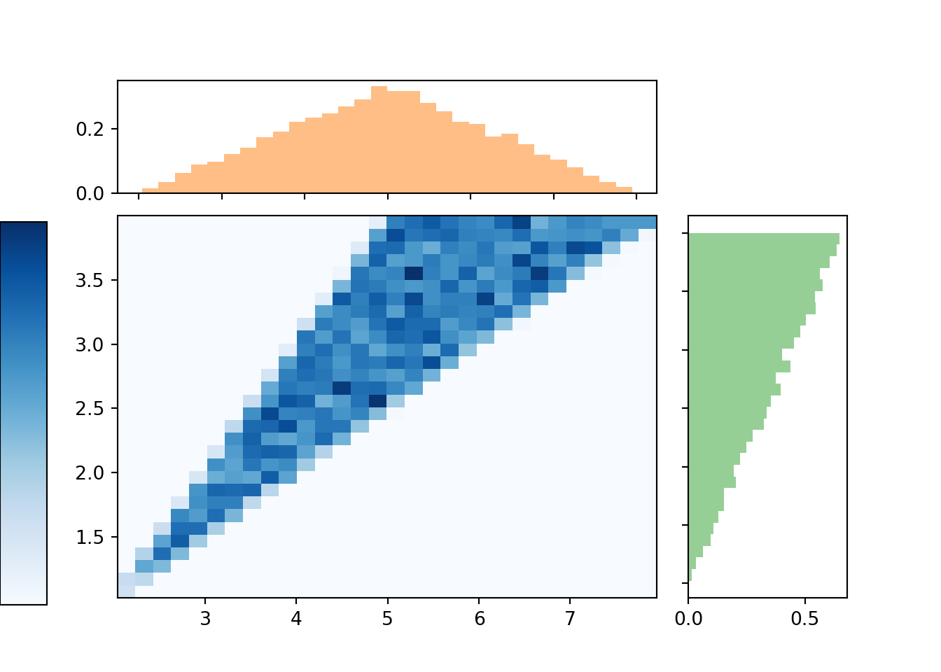

Let’s look a little more closely at the marginal distribution of $X$.

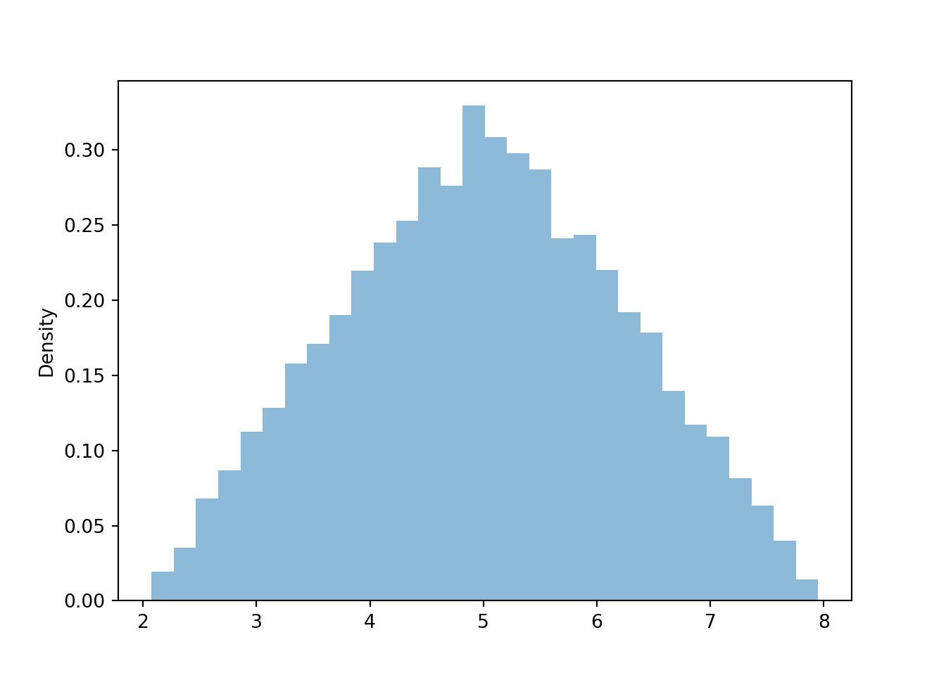
$Histogram representing the marginal distribution of the sum ($X$) of two spins of the Uniform(1, 4) spinner.$

Figure 4.10: Histogram representing the marginal distribution of the sum ($X$) of two spins of the Uniform(1, 4) spinner.

The marginal distribution of $X$ has highest density near 5 and lowest density near 2 and 8. Intuitively, there is only one pair of spins — (1, 1) — for which the sum is 2; similarly for a sum of 8. But there are many pairs for which the sum is 5: (2.5, 2.5), (3, 2), (2, 3), (1.2, 2.8), etc. Recall that for the dice rolls, we could obtain the marginal distribution of $X$ by summing the joint distribution over all $Y$ values. Similarly, we can find the marginal density of $X$ by aggregating over all possible values of $Y$. For each possible value of $X$, “collapse” the joint histogram vertically over all possible values of $Y$. Imagine that within the region of possible $(X, Y)$ pairs, the joint histogram is composed of stacks of blocks, one for each bin, each stack of the same height (because the values are uniformly distributed over the triangular region). To get the marginal density for a particular $x$, take all the stacks corresponding to that $x$, for different values of $y$, and stack them on top of one another. There will be the most stacks for $x$ values near 5 and the fewest stacks for $x$ values near 2 or 8. In other words, the aggregated density along “vertical strips” is largest for the vertical strip for $x=5$. (In this case, the joint distribution is uniform over the range of possible pairs, so the stacks all have the same height. That won’t be true in general, so the marginal distributions will depend both on the number of and the height of the “stacks”.)

Similarly reasoning applies to find the marginal distribution of $Y$. Now we find the marginal density for a particular $y$ value by collapsing/stacking the histogram horizontally over all possible value of $X$. We see that the density increases with values of $y$. Intuitively, there is only one pair of spins, (1, 1), for which $Y=1$, but many pairs of spins for which $Y=4$, e.g., (1, 4), (4, 1), (4, 2), (2.5, 4), etc.

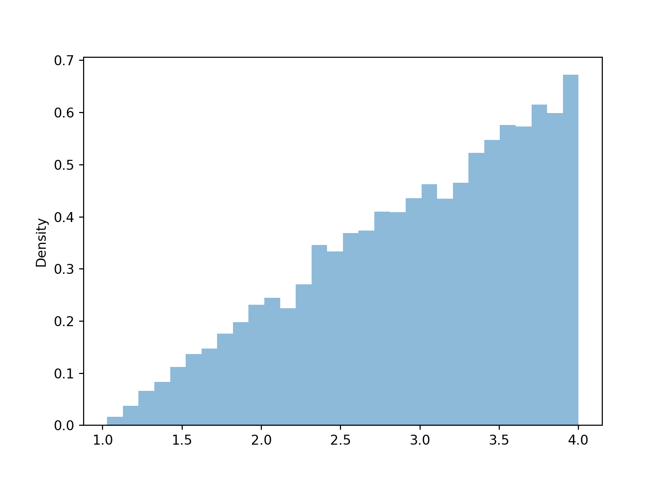
$Histogram representing the marginal distribution of the larger ($Y$) of two spins of the Uniform(1, 4) spinner.$

Figure 4.11: Histogram representing the marginal distribution of the larger ($Y$) of two spins of the Uniform(1, 4) spinner.

What about the long run averages? The sums of the two spins is $X= U_1 + U_2$. The long run average of each of $U_1$ and $U_2$ is 2.5 (the midpoint of the interval [1, 4]). We can see from its marginal distribution that the long run average of $X$ is 5. Therefore, the average of the sum is the sum of averages.


X.sim(10000).mean()

## 4.972145474305705

However, the average of $Y=\max(U_1, U_2)$ is 3, which is not $\max(2.5, 2.5)$. Therefore, the average of the maximum is not the maximum of the averages. Remember that in general, Average of $g(X, Y)$ $\neq$ $g$(Average of $X$, Average of $Y$).


Y.sim(10000).mean()

## 3.005660101873536

Finally, observe that the plots in this section look like continuous versions of the plots for the dice rolling example earlier in the chapter. However, it took a little more work in this section to think about what the joint or marginal distributions might look like. When studying continuous random variables, it is often helpful to think about how a discrete analog behaves.

4.9.1 Summary

The joint distribution of values on a continuous scale can be visualized in a joint histogram.
Remember to always identify possible values of random variables, including possible pairs in a joint distribution.
The marginal distribution of a single random variable can be obtained from a joint distribution by aggregating/collapsing/stacking over the values of the other random variables.
The average of a sum is the sum of the averages. Whether in the short run or the long run, \[\begin{align*} \text{Average of $X+Y$} & = \text{Average of $X$} +\text{Average of $Y$} \end{align*}\]
Whether in the short run or the long run, in general: Average of $g(X, Y)$ $\neq$ $g$(Average of $X$, Average of $Y$).
When studying continuous random variables, it is often helpful to think about how a discrete analog behaves.

4.9.2 Exercises

Exercise 4.1 Spin the Uniform(0, 1) spinner twice and let $U_1$ and $U_2$ be the result of the two spins. Each of the following random variables takes values in the interval (-1, 1). (You should verify this.)

$V = 2 U_1 - 1$.
$W = 2U_1^2 - 1$.
$U_1^2$ the square of $U_1$.
$X = U_1 - U_2$.
$Y = 2\max(U_1, U_2) - 1$.
$Z = (2 U_1 - 1)^{1/3}$, where the cube root of a negative number is defined to be negative, e.g. $(-1/8)^{1/3} = -1/2$; $(-1)^{1/3} = -1$.

Match each of the random variables above with the feature below that best describes its distribution. Each feature will be used exactly once.

Density is uniform over $(-1, 1)$.
Density is highest at -1 and lowest at 1.
Density is highest at 0 and lowest at -1 and 1.
Density is highest at 1 and lowest at -1.
Density is highest at 1 and -1 and lowest at 0.

Hint: It helps to sketch plots and work out what happens for a few example intervals (e.g. (0, 0.1), (0.1, 0.2)). You can also use simulation to see what happens, but try sketching a plot first to practice your understanding.

Remember that a probability space outcome corresponds to the pair of spins, so we can define random variables on this space as we have done. We could also first define random variables U1, U2 = RV(P) corresponding to the individual spins, and then define the sum as X = U1 + U2. For technical reasons the syntax for max is a little different: Y = (U1 & U2).apply(max).↩︎