2.5 Computer simulation: Symbulate
Note: some of the plots and tables in this and the following sections do not appear exactly as they would in Jupyter or Colab notebooks. See the accompanying notebooks for a better representation of Symbulate output.
We will perform computer simulations using the Python package Symbulate. The syntax of Symbulate mirrors the language of probability in that the primary objects in Symbulate are the same as the primary components of a probability model: probability spaces, random variables, events. Once these components are specified, Symbulate allows users to simulate many times from the probability model and summarize the results.
This section contains a brief introduction to Symbulate; many more examples can be found throughout the text or in the Symbulate documentation. Remember to first import Symbulate during a Python session using the command
from symbulate import *Throughout Section 2.5 we illustrate Symbulate commands and output in the context of Example 2.2 from Section 2.2. Unless indicated otherwise, in this section \(X\) represents the sum of two rolls of a fair four-sided die, and \(Y\) represents the larger of the two rolls (or the common value if a tie). We have already discussed the simulation process in this situation. Now we have to implement that process on a computer.
2.5.1 Simulating outcomes
The following Symbulate code defines a probability space29 P for simulating the 16 equally likely ordered pairs of rolls via a box model.
P = BoxModel([1, 2, 3, 4], size = 2, replace = True)The above code tells Symbulate to draw 2 tickets (size = 2), with replacement30, from a box with tickets labeled
1, 2, 3, and 4 (entered as the Python list [1, 2, 3, 4]). Each simulated outcome consists of an ordered31 pair of rolls. The sim(n) command simulates n realizations of probability space outcomes (or events or random variables).
P.sim(10)| Index | Result |
|---|---|
| 0 | (3, 2) |
| 1 | (2, 4) |
| 2 | (3, 1) |
| 3 | (1, 2) |
| 4 | (3, 1) |
| 5 | (4, 2) |
| 6 | (1, 2) |
| 7 | (2, 3) |
| 8 | (3, 4) |
| ... | ... |
| 9 | (1, 4) |
2.5.2 Simulating random variables
A Symbulate RV is specified by the probability space on which it is defined and the mapping function which defines it. Recall that \(X\) is the sum of the two dice rolls and \(Y\) is the larger (max).
X = RV(P, sum)
Y = RV(P, max)
The above code simply defines the random variables. Since a random variable \(X\) is a function, any RV can be called as a function32 to return its value \(X(\omega)\) for a particular outcome \(\omega\) in the probability space.
omega = (3, 2)  # a pair of rolls
X(omega), Y(omega)
## Warning: Calling an RV as a function simply applies the function that defines the RV to the input, regardless of whether that input is a possible outcome in the underlying probability space.
## Warning: Calling an RV as a function simply applies the function that defines the RV to the input, regardless of whether that input is a possible outcome in the underlying probability space.
## (5, 3)The following commands simulate 100 values of the random variable Y and store the results as y. For consistency with standard probability notation33, the random variable itself is denoted with an uppercase letter Y, while the realized values of it are denoted with a lowercase letter y.
y = Y.sim(100)
y # this just diplays y| Index | Result |
|---|---|
| 0 | 2 |
| 1 | 2 |
| 2 | 4 |
| 3 | 4 |
| 4 | 4 |
| 5 | 4 |
| 6 | 3 |
| 7 | 2 |
| 8 | 2 |
| ... | ... |
| 99 | 4 |
2.5.3 A few commands for summarizing simulation output
Values and their frequencies can be summarized using tabulate.
y.tabulate()| Value | Frequency |
|---|---|
| 1 | 5 |
| 2 | 23 |
| 3 | 28 |
| 4 | 44 |
| Total | 100 |
By default, tabulate returns frequencies (counts). Adding the argument34 normalize = True returns relative frequencies (proportions).
y.tabulate(normalize = True)| Value | Relative Frequency |
|---|---|
| 1 | 0.05 |
| 2 | 0.23 |
| 3 | 0.28 |
| 4 | 0.44 |
| Total | 1.0 |
Methods like sim and tabulate can be chained together in a single line of code.
Y.sim(100).tabulate(normalize = True)| Value | Relative Frequency |
|---|---|
| 1 | 0.04 |
| 2 | 0.22 |
| 3 | 0.28 |
| 4 | 0.46 |
| Total | 1.0 |
Each call to sim reruns the simulation to generate a new set of simulated values. To perform multiple operations on a single set of simulated values, store the simulation results as a variable (like y above). When running Y.sim(100) Symbulate simulates, in the background, outcomes from the probability space P and then computes Y for these outcomes; however, the outcomes themselves are not saved. (We will soon see how to simulate multiple quantities simultaneously.)
The tabulate method provides a quick summary of the individual simulated values and their frequencies. We can find frequencies of other events using the “count” functions:
count_eq(u): count equal to ucount_neq(u): count not equal to ucount_leq(u): count less than or equal to ucount_lt(u): count less than ucount_geq(u): count greater than or equal to ucount_gt(u): count greater than ucount: count according to a specified True/False criteria. (See the code after Figure 2.8 for an example.) Note:count()with no inputs to defaults to “count all”.
y.count()## 100y.count_eq(3) / y.count()## 0.28y.count_leq(3) / y.count()## 0.56Graphical summaries play an important role in describing distributions. We can plot the 100 individual simulated values of \(Y\) in a rug plot.
y.plot('rug')
plt.show()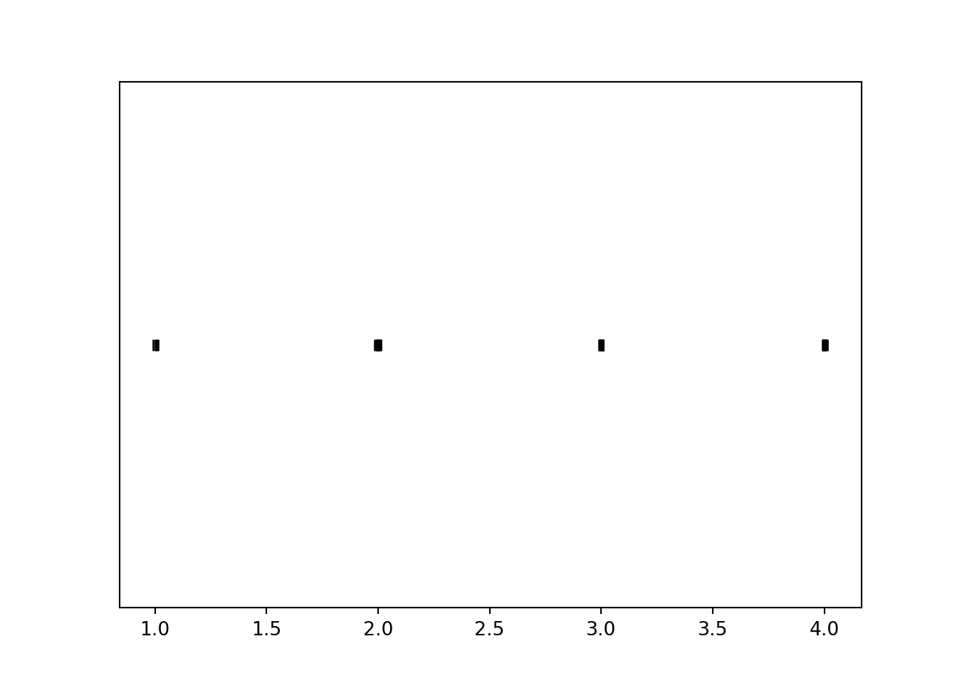
The rug plot emphasizes that realizations of the random varible \(Y\) are numbers along a number line. However, the rug plot does not adequately summarize the relative frequencies. Instead, calling .plot() produces35 an impulse plot which displays the simulated values and their relative frequencies.
y.plot()
plt.show()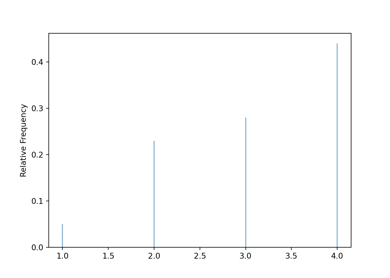
We will introduce several more plot types and commands for summarizing simulation output in the following sections.
2.5.4 Approximating probabilities and distributions
The theoretical distribution of \(Y\) in the die rolling example is represented by Table ??. The plot above, based on only 100 simulated values, provides a poor approximation to the distribution of \(Y\). We often initially simulate a small number of repetitions to see what the simulation is doing and check that it is working properly. However, in order to accurately approximate probabilities or distribution we simulate a large number of repetitions (usually thousands for our purposes).
Now we simulate 10,000 values of the random variable Y and summarize the simulation output to approximate the distribution of \(Y\). Since the simulation results below are stored as y, the same set of results is used to produce the table and the plot. Compare the simulation results summarized in Figure 2.5 with Table ??. The results of 10000 repetitions provide a much better approximation to the true distribution of \(Y\) than the results of just 100 repetitions.
y = Y.sim(10000)
y.tabulate()| Value | Frequency |
|---|---|
| 1 | 619 |
| 2 | 1882 |
| 3 | 3134 |
| 4 | 4365 |
| Total | 10000 |
y.plot()
plt.show()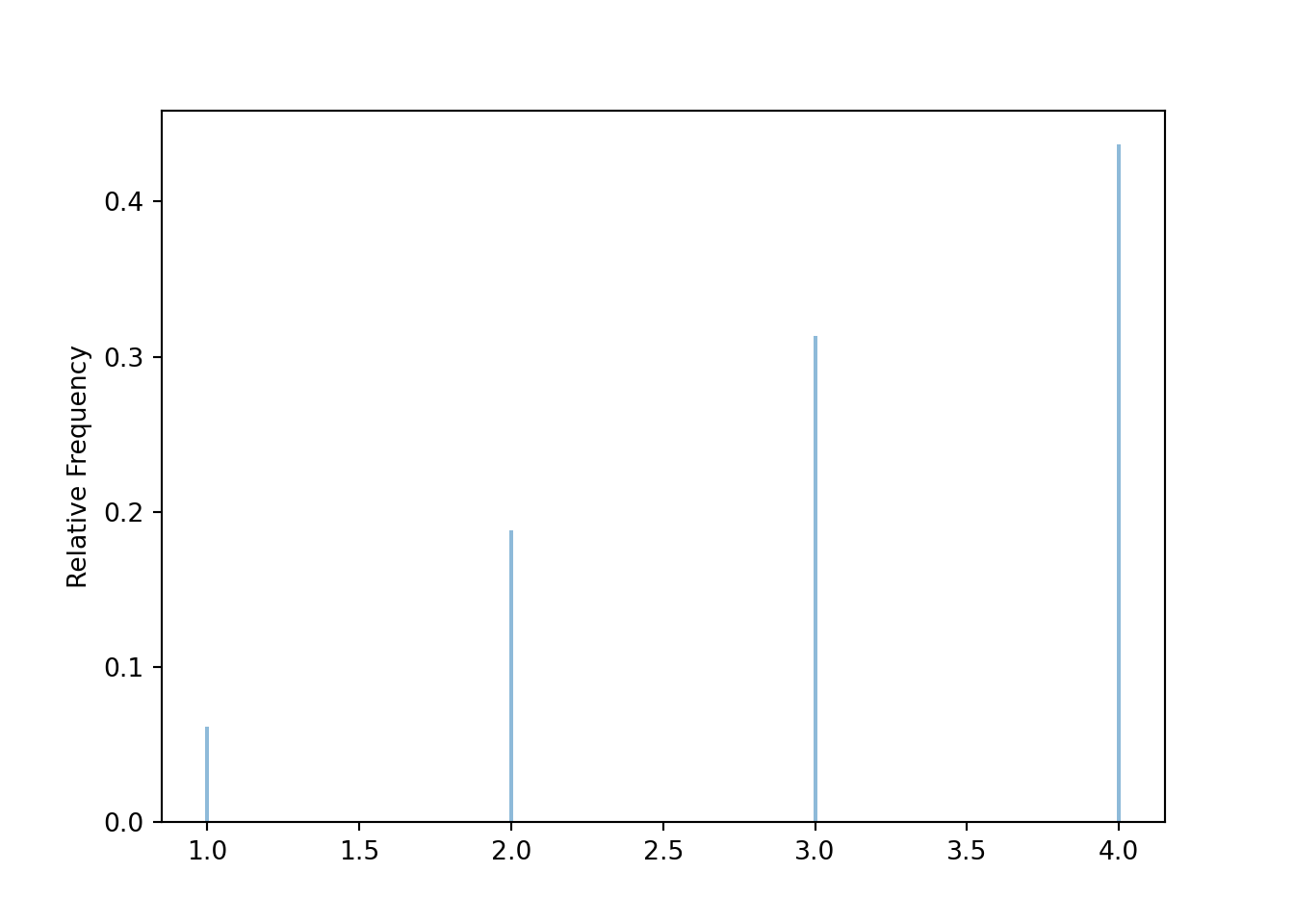
Figure 2.5: Simulation-based approximate distribution of \(Y\), the larger (or common value if a tie) of two rolls of a fair four-sided die.
Figure 2.6 contains a summary of a simulated \(X\) values. Compare with Table ??.
x = X.sim(10000)
x.tabulate(normalize = True)| Value | Relative Frequency |
|---|---|
| 2 | 0.0566 |
| 3 | 0.1174 |
| 4 | 0.1929 |
| 5 | 0.2611 |
| 6 | 0.1896 |
| 7 | 0.1221 |
| 8 | 0.0603 |
| Total | 1.0 |
x.plot()
plt.show()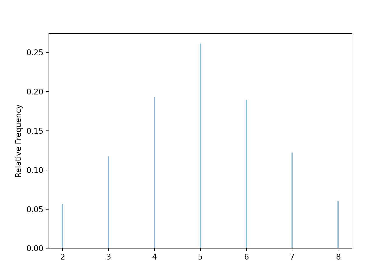
Figure 2.6: Simulation-based approximate distribution of \(X\), the sum of two rolls of a fair four-sided die.
Since probabilities can be interpreted as long run relative frequencies, we can use simulate many repetitions and use the count functions to compute relative frequencies and approximate probabilities of events.
y.count()## 10000y.count_eq(3) / y.count()## 0.3134y.count_leq(3) / y.count()## 0.56352.5.5 Approximating long run averages
Recall that we have stored 10000 simulated values of \(Y\) as y. We can approximate the long run average value of \(Y\) by computing the average — a.k.a., mean — of the 10000 simulated values in the usual way: sum the 10000 simulated values stored in y and divide by 10000. Here are a few ways of computing the mean of the simulated values.
y.sum() / 10000## 3.1245
y.sum() / y.count()## 3.1245
y.mean()## 3.1245Similarly, the approximate long run average value of \(X\) is
x.mean()## 5.0172These values represent the “balance points” in Figure 2.5 and Figure 2.6. We will discuss long run average values in more detail later.
2.5.6 Simulating events
So far, we have simulated values of random variables and used the results to approximate probabilities of related events. Events can also be defined and simulated directly.
For programming reasons, events are enclosed in parentheses () rather than braces \(\{\}\). For example, we can define the event that the larger of the two rolls is less than 3, \(A=\{Y<3\}\), as
A = (Y < 3) # an eventWe can use sim to simulate events.
A realization of an event is True if the event occurs for the simulated outcome, or False if not.
A.sim(10)| Index | Result |
|---|---|
| 0 | False |
| 1 | False |
| 2 | True |
| 3 | False |
| 4 | True |
| 5 | False |
| 6 | False |
| 7 | True |
| 8 | False |
| ... | ... |
| 9 | False |
For logical equality use a double equal sign ==. For example, (Y == 3) represents the event \(\{Y=3\}\).
(Y == 3).sim(10000).tabulate()| Outcome | Frequency |
|---|---|
| False | 6871 |
| True | 3129 |
| Total | 10000 |
Since event \(A\) is defined in terms of \(Y\), we can also first simulate values of \(Y\), store the results, and then determine whether event \(A\) occurs based on each of the simulated values of \(Y\). (The following code uses the values of y we had simulated earlier, and so will not match the output of the code above.)
(y == 3)| Index | Result |
|---|---|
| 0 | False |
| 1 | True |
| 2 | False |
| 3 | False |
| 4 | False |
| 5 | False |
| 6 | True |
| 7 | False |
| 8 | True |
| ... | ... |
| 9999 | False |
(y == 3).count_eq(True) / y.count()## 0.3134Python automatically treats True as 1 and False as 0, so the code (Y == 3) functions effectively both as the event itself and as the indicator random variable for the event.
In particular, we can count the number of repetitions on which the event occurs by summing the simulated values of the indicator.
(y == 3).sum() / y.count()## 0.31342.5.7 Simulating multiple random variables
We can simulate \((X, Y)\) pairs using36 &. We store the simulation output as xy to emphasize that xy contains pairs of values.
xy = (X & Y).sim(10000)
xy| Index | Result |
|---|---|
| 0 | (8, 4) |
| 1 | (7, 4) |
| 2 | (5, 4) |
| 3 | (6, 3) |
| 4 | (4, 2) |
| 5 | (2, 1) |
| 6 | (5, 3) |
| 7 | (6, 4) |
| 8 | (6, 3) |
| ... | ... |
| 9999 | (6, 4) |
Pairs of values can also be tabulated.
xy.tabulate()| Value | Frequency |
|---|---|
| (2, 1) | 585 |
| (3, 2) | 1272 |
| (4, 2) | 642 |
| (4, 3) | 1215 |
| (5, 3) | 1239 |
| (5, 4) | 1310 |
| (6, 3) | 648 |
| (6, 4) | 1271 |
| (7, 4) | 1243 |
| (8, 4) | 575 |
| Total | 10000 |
xy.tabulate(normalize = True)| Value | Relative Frequency |
|---|---|
| (2, 1) | 0.0585 |
| (3, 2) | 0.1272 |
| (4, 2) | 0.0642 |
| (4, 3) | 0.1215 |
| (5, 3) | 0.1239 |
| (5, 4) | 0.131 |
| (6, 3) | 0.0648 |
| (6, 4) | 0.1271 |
| (7, 4) | 0.1243 |
| (8, 4) | 0.0575 |
| Total | 1.0 |
Individual pairs can be plotted in a scatter plot, which is a two-dimensional analog of a rug plot.
xy.plot()
plt.show()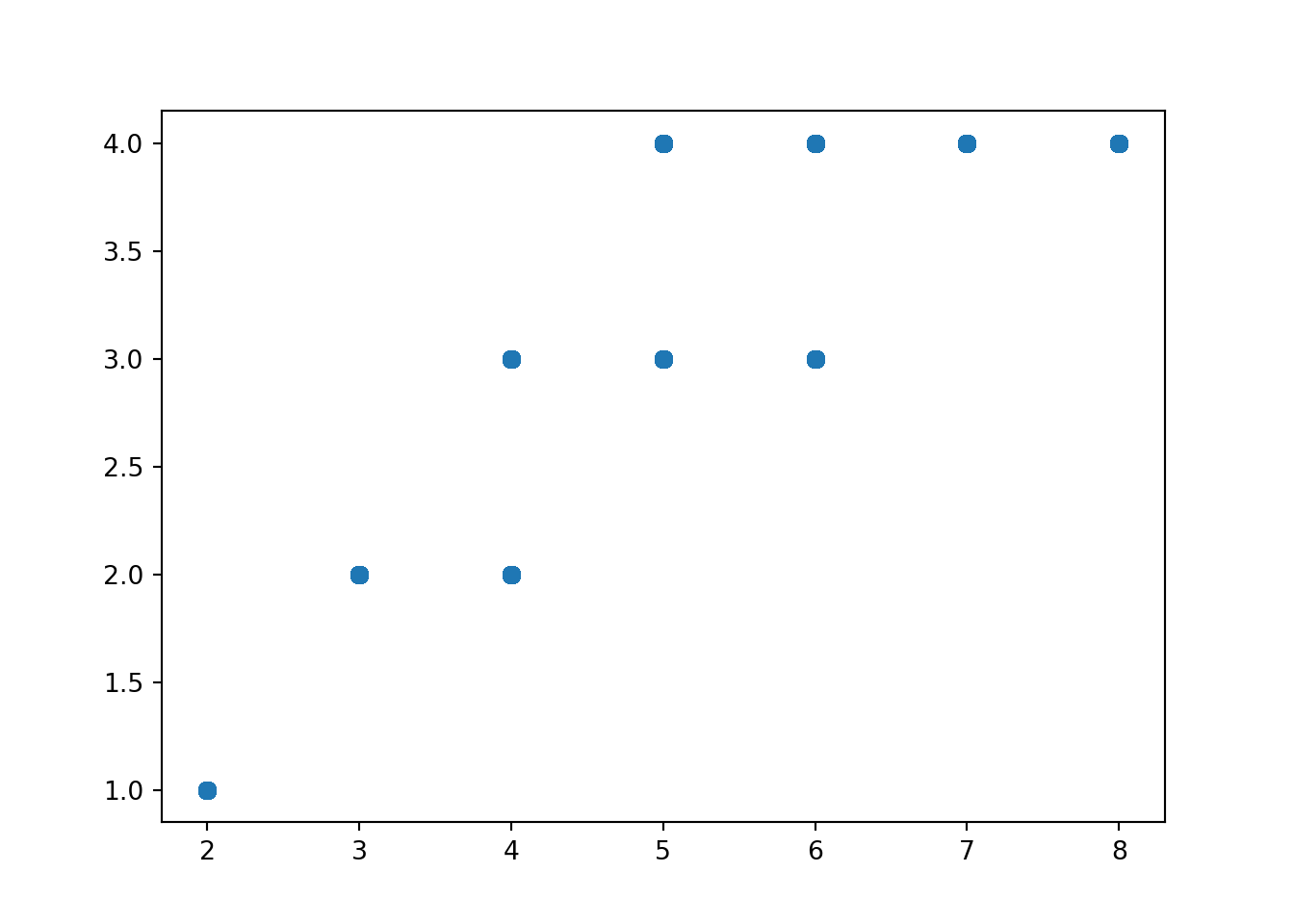
The values can be “jittered” slightly, as below, so that points do not coincide.
xy.plot(jitter = True)
plt.show()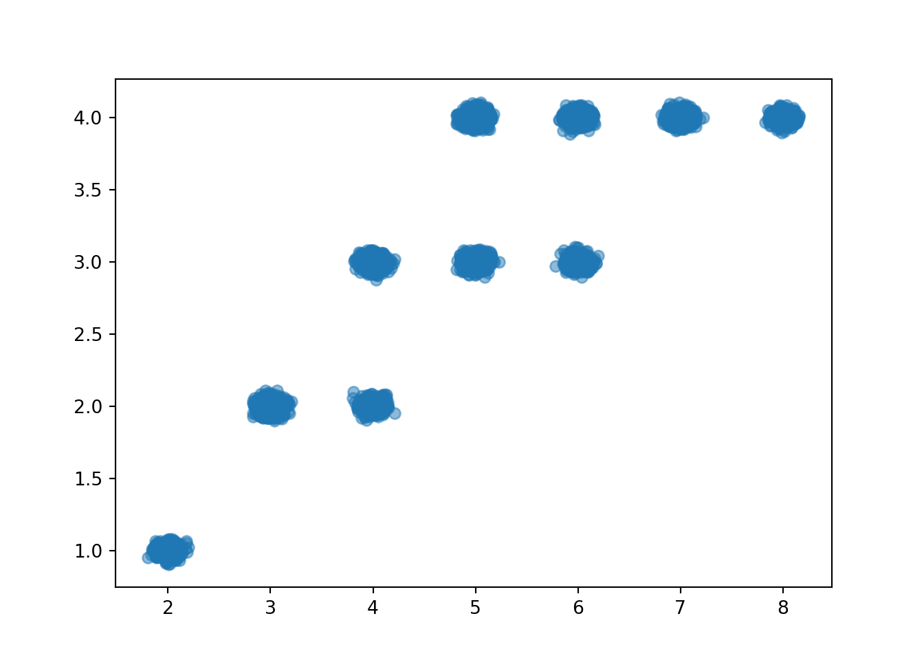
Even with jittering, the scatter plot does not adequately represent relative frequencies.
The two-dimensional analog of an impulse plot is a tile plot. For two discrete variables, the 'tile' plot type produces a tile plot (a.k.a. heat map) where rectangles represent the simulated pairs with their relative frequencies visualized on a color scale.
xy.plot('tile')
plt.show()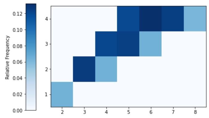
Figure 2.7: Tile plot visualization of the simulation-based approximate joint distribution of the sum (\(X\)) and larger (\(Y\)) of two rolls of a fair four-sided die. Color intensity represents relative frequencies of pairs.
We can add the impulse plot for each of \(X\) and \(Y\) in the margins of the tile plot using the 'marginal' argument.
xy.plot(['tile', 'marginal'])
plt.show()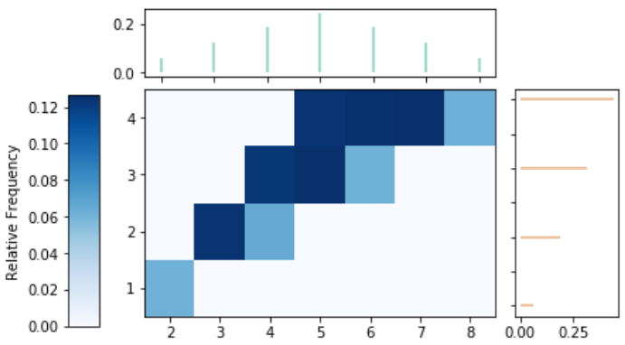
Figure 2.8: Tile and impulse plot visualization of the simulation-based approximate joint and marginal distributions of the sum (\(X\)) and larger (\(Y\)) of two rolls of a fair four-sided die.
Custom functions can be used with count to compute relative frequencies of events involving multiple random variables. Suppose we want to approximate \(\textrm{P}(X<6, Y \ge 2)\). We first define a Python function which takes as an input a pair u = (u[0], u[1]) and returns True if u[0] < 6 and u[1] >= 2.
def is_x_lt_6_and_y_ge_2(u):
  if u[0] < 6 and u[1] >= 2:
    return True
  else:
    return False
Now we can use this function along with count to find the simulated relative frequency of the event \(\{X <6, Y \ge 2\}\).
Remember that xy stores \((X, Y)\) pairs of values, so the first coordinate xy[0] represents values of \(X\) and the second coordinate xy[1] represents values of \(Y\).
xy.count(is_x_lt_6_and_y_ge_2) / xy.count()## 0.5678We could also count use Boolean logic; basically using indicators and the property \(\textrm{I}_{\{X<6,Y\ge 2\}}=\textrm{I}_{\{X<6\}}\textrm{I}_{\{Y\ge 2\}}\).
((xy[0] < 6) * (xy[1] >= 2)).count_eq(True) / xy.count()## 0.56782.5.8 Simulating outcomes and random variables
Recall Table 2.3 which displays both the outcomes of the two rolls and the corresponding values of \(X\) and \(Y\) for 10 repetitions. Calling (X & Y).sim(10) as in the previous section produces results like those in the table, but only the values of (X & Y) are saved and displayed. The outcomes of the rolls are generated in the background but not saved.
We can create a RV which returns the outcomes of the probability space37. The default mapping function for RV is the identity function, \(g(u) = u\), so simulating values of U = RV(P) below returns the outcomes of the BoxModel P representing the outcome of the two rolls.
U = RV(P)
U.sim(10)| Index | Result |
|---|---|
| 0 | (3, 2) |
| 1 | (1, 3) |
| 2 | (4, 2) |
| 3 | (2, 2) |
| 4 | (2, 1) |
| 5 | (3, 3) |
| 6 | (2, 4) |
| 7 | (3, 2) |
| 8 | (4, 2) |
| ... | ... |
| 9 | (1, 3) |
Now we can simulate and display the outcomes along with the values of \(X\) and \(Y\) using &.
(U & X & Y).sim(10)| Index | Result |
|---|---|
| 0 | ((1, 2), 3, 2) |
| 1 | ((1, 2), 3, 2) |
| 2 | ((4, 2), 6, 4) |
| 3 | ((3, 2), 5, 3) |
| 4 | ((1, 3), 4, 3) |
| 5 | ((2, 4), 6, 4) |
| 6 | ((2, 3), 5, 3) |
| 7 | ((2, 1), 3, 2) |
| 8 | ((4, 3), 7, 4) |
| ... | ... |
| 9 | ((3, 3), 6, 3) |
Because the probability space P returns pairs of values, U = RV(P) above defines a random vector. The individual components38 of U can be “unpacked” as U1, U2 in the following. Here U1 represents the result of the first roll and U2 the second.
U1, U2 = RV(P)
(U1 & U2 & X & Y).sim(10)| Index | Result |
|---|---|
| 0 | (2, 3, 5, 3) |
| 1 | (2, 4, 6, 4) |
| 2 | (2, 3, 5, 3) |
| 3 | (2, 3, 5, 3) |
| 4 | (2, 3, 5, 3) |
| 5 | (1, 1, 2, 1) |
| 6 | (2, 1, 3, 2) |
| 7 | (3, 2, 5, 3) |
| 8 | (1, 2, 3, 2) |
| ... | ... |
| 9 | (4, 4, 8, 4) |
2.5.9 Transformations of random variables
Transformations of random variables are random variables.
If X is a Symbulate RV and g is a function, then g(X) is also a Symbulate RV.
For example, we can approximate the long run average value of \(X^2\).
(X ** 2).sim(10000).mean()## 27.5402For many common functions, the syntax g(X) is sufficient.
Here exp(u) is the exponential function \(g(u) = e^u\).
(X & exp(X)).sim(10)| Index | Result |
|---|---|
| 0 | (8, 2980.9579870417283) |
| 1 | (7, 1096.6331584284585) |
| 2 | (3, 20.085536923187668) |
| 3 | (6, 403.4287934927351) |
| 4 | (8, 2980.9579870417283) |
| 5 | (4, 54.598150033144236) |
| 6 | (5, 148.4131591025766) |
| 7 | (5, 148.4131591025766) |
| 8 | (4, 54.598150033144236) |
| ... | ... |
| 9 | (7, 1096.6331584284585) |
For user defined functions, the syntax is X.apply(g).
def g(u):
  return (u - 5) ** 2

Z = X.apply(g)

(X & Z).sim(10)| Index | Result |
|---|---|
| 0 | (3, 4) |
| 1 | (6, 1) |
| 2 | (5, 0) |
| 3 | (2, 9) |
| 4 | (5, 0) |
| 5 | (6, 1) |
| 6 | (2, 9) |
| 7 | (2, 9) |
| 8 | (4, 1) |
| ... | ... |
| 9 | (4, 1) |
(We could have actually defined Z = (X - 5) ** 2 here.
We’ll see examples where the apply syntax is necessary later.)
We can also apply transformations of multiple RVs defined on the same probability space.
(We will look more closely at how Symbulate treats this “same probability space” issue later.)
For example, we can approximate the long run average value of \(XY\).
(X * Y).sim(10000).mean()## 16.9367Recall that we defined \(X\) via X = RV(P, sum).
Defining random variables \(U_1, U_2\) to represent the individual rolls, we can define \(X=U_1 + U_2\).
Recall that we defined39 U1, U2 = RV(P).
X = U1 + U2

X.sim(10000).tabulate(normalize = True)| Value | Relative Frequency |
|---|---|
| 2 | 0.0666 |
| 3 | 0.1239 |
| 4 | 0.1856 |
| 5 | 0.2534 |
| 6 | 0.184 |
| 7 | 0.1233 |
| 8 | 0.0632 |
| Total | 0.9999999999999999 |
Unfortunately max(U1, U2) does not work, but we can use the apply syntax.
Since we want to apply max to \((U_1, U_2)\) pairs, we must40 first join them together with &.
Y  = (U1 & U2).apply(max)

Y.sim(10000).tabulate(normalize = True)| Value | Relative Frequency |
|---|---|
| 1 | 0.0639 |
| 2 | 0.1847 |
| 3 | 0.3173 |
| 4 | 0.4341 |
| Total | 1.0 |
2.5.10 Two “worlds” in Symbulate
In Section 2.5.6 we saw that we could either
- Define the event
(Y < 3)and simulate True/False realizations of it, or - Define the random variable
Y, simulate values of it and store them asy, and then evaluate the event for each of the simulated values with(y < 3).
These two methods illustrate the two “worlds” of Symbulate, which we call “random variable world” and “simulation world”.
Operations like transformations can be performed in either world.
Think of random variable world as the “before” world and simulation world as the “after” world, by which we mean before/after the sim step.
Most of the transformations we have seen so far happened in random variable world. For example, we have seen how to define the sum of two dice in random variable world in a few ways, e.g., via
P = BoxModel([1, 2, 3, 4], size = 2)
U = RV(P)

X = U.apply(sum)
The sum transformation is applied to define a new random variable X, before the sim step.
We could then call, e.g., (U & X).sim(10000).
We could also compute simulated values of the sum in simulation world as follows.
P = BoxModel([1, 2, 3, 4], size = 2)
U = RV(P)

u = U.sim(10000)

x = u.apply(sum)
The above code will simulate all the pairs of rolls first, store them as u, and then apply the sum to the simulated values.
That is, the sum transformation happens after the sim step.
While either world is “correct”, we generally take the random variable world approach. We do this mostly for consistency, but also to emphasize some of the probability concepts we’ll encounter. For example, the fact that a sum of random variables (defined on the same probability space) is also a random variable is a little more apparent in random variable world. However, it is sometimes more convenient to code in simulation world; for example, if complicated transformations are required.
When working in random variable world, it only makes sense to transform random variables defined on the same probability space.
Likewise, in simulation world, it only makes sense to apply transformations to values generated in the same simulation, with a single sim step.
For example, the following code would return an error.
P = BoxModel([1, 2, 3, 4], size = 2)
U1, U2 = RV(P)

u1 = U1.sim(10000)
u2 = U2.sim(10000)

x = u1 + u2 # returns an error: "objects must come from the same simulation"
We’ll discuss the reason for this error in more detail later.
In short, the “simulation” step should be implemented in a single call to sim.
2.5.11 Brief summary of Symbulate commands
This section has only presented an introduction to simulations and Symbulate. We will see many more scenarios and additional Symbulate commands throughout the book.
Many scenarios require only a few lines of Symbulate code to set up, run, analyze, and visualize. The following table comprises the requisite Symbulate commands for a wide variety of situations.
| Command | Function |
|---|---|
BoxModel |
Define a box model |
ProbabilitySpace |
Define a custom probability space |
RV |
Define random variables, vectors, or processes |
RandomProcess |
Define a discrete or continuous time stochastic process |
apply |
Apply transformations |
[] (brackets) |
Access a component of a random vector, or a random process at a particular time |
* (and **) |
Define independent probability spaces or distributions |
AssumeIndependent |
Assume random variables or processes are independent |
| (vertical bar) |
Condition on events |
& |
Join multiple random variables into a random vector |
sim |
Simulate outcomes, events, and random variables, vectors, and processes |
tabulate |
Tabulate simulated values |
plot |
Plot simulated values |
filter (and relatives) |
Create subsets of simulated values (filter_eq, filter_lt, etc) |
count (and relatives) |
Count simulated values which satisfy some critera (count_eq, count_lt, etc) |
| Statistical summaries | mean, median, sd, var, quantile, corr, cov, etc. |
| Common models | See later |
While no previous experience with Python is required, it is also possible to incorporate Python programming with Symbulate code. In particular, Python functions or loops can be used: to define or transform random variables or stochastic processes, or to investigate the effects of changing parameter values. Also, while many common plots are built in with the Symbulate plot function, the Matplotlib package can be used to create or customize plots. Some of these features will be illustrated in the next section and more examples are found throughout the text.
2.5.12 Exercises
Flip a fair coin 4 times and let \(X\) be the number of H.
- Write the Symbulate code to define \(X\) using a box model with tickets labeled H and T. Simulate a few outcomes and a few values of \(X\).
- Write the Symbulate code to define \(X\) using a box model with tickets labeled 1 and 0 and without counting. Simulate a few outcomes together with their values of \(X\).
- Write the Symbulate code to conduct a simulation and use the results to approximate \(\textrm{P}(X = 3)\).
Technically, a probability space is a triple \((\Omega, \mathcal{F}, \textrm{P})\). We primarily view a Symbulate probability space as a description of the probability model rather than an explicit specification of \(\Omega\). For example, we define a
BoxModelinstead of creating a set with all possible outcomes. We tend to represent a probability space withP, even though this is a slight abuse of notation.↩︎The default argument for
replaceisTrue, so we could have just writtenBoxModel([1, 2, 3, 4], size = 2).↩︎There is an additional argument
order_matterswhich defaults toTrue, but we could set it to false for unordered pairs.↩︎The warning you get when you call a
RVas a function just means that Symbulate is not going to check for you that the inputs to the function you used to define theRVactually match up with the outcomes of the probability spaceP.↩︎We generally use names in our code that mirror and reinforce standard probability notation, e.g., uppercase letters near the end of the alphabet for random variables, with corresponding lowercase letters for their realized values. Of course, these naming conventions are not necessary and you are welcome to use more descriptive names in your code. For example, we could have named the probability space
DiceRollsand the random variablesDiceSumandDiceMaxrather thanP, X, Y.↩︎“Normalize” is used in the sense of Section 1.3 and refers to rescaling the values so that they add up to 1 but the ratios are preserved.↩︎
For discrete random variables
'impulse'is the default plot type. Like.tabulate(), the.plot()method also has anormalizeargument; the default isnormalize=True.↩︎Technically
&joins twoRVs together to form a random vector. While we often interpret SymbulateRVas random variable, it really functions as random vector.↩︎You might try
(P & X).sim(10). ButPis a probability space object, andXis anRVobject, and&can only be used to join like objects together. Much like in probability theory in general, in Symbulate the probability space plays a background role, and it is usually random variables we are interested in.↩︎The components can also be accessed using brackets.
U1, U2 = RV(P)is shorthand for
U = RV(P); U1 = U[0]; U2 = U[1]. Python uses zero-based indexing, so 0 refers to the first component, 1 to the second, and so on.↩︎We can also define
U = RV(P)and thenX = U.apply(sum).↩︎We can also define
U = RV(P)and thenX = U.apply(max).↩︎