4.10 Joint Normal Distributions
In previous sections we considered randomly selecting an SAT taker and measuring their Math score. In particular, we assumed that SAT Math scores follow a Normal distribution with a mean of 500 and a standard deviation of 100.
Now consider randomly selecting an SAT taker and recording both their Math and Reading score. Suppose we want to conduct an appropriate simulation.
Example 4.10 Donny Don’t says: “That’s easy; just spin the SAT spinner twice, once for Math and once for Reading.” Do you agree? Explain your reasoning.
Solution. to Example 4.10
Show/hide solution
You should not agree with Donny, for two reasons.
- It’s possible that the distribution of SAT Math scores follow a different pattern than SAT Reading scores. So we might need one spinner to simulate a Math score, and a second spinner to simulate the Reading score. (In reality, SAT Math and Reading scores do follow pretty similar distributions. But it’s possible that they could follow different distributions.)
- Furthermore, there is probably some relationship between scores. It is plausible that students who do well on one test tend to do well on the other. For example, students who score over 700 on Math are probably more likely to score above than below average on Reading. If we simulate a pair of scores by spinning one spinner for Math and a separate spinner for Reading, then there will be no relationship between the scores because the spins are physically independent.
What we really need is a spinner that generates a pair of scores simultaneously to reflect their association. This is a little harder to visualize, but we could imagine spinning a “globe” with lines of latitude corresponding to SAT Math score and lines of longitutde to SAT Reading score. But this would not be a typical globe:
- The lines of latitude would not be equally spaced, since SAT Math scores are not equally likely. (We have seen similar issues for one-dimensional spinners like the one in Figure ?? with unequally spaced values around the outside.) Similarly for lines of longitude.
- The scale of the lines of latitude would not necessarily match the scale of the lines of longitude, since Math and Reading scores could follow difference distributions. For example, the equator (average Math) might be 500 while the prime meridian (average Reading) might be 520.
- The “lines” would be tilted or squiggled to reflect the relationship between the scores. For example, the region corresponding to Math scores near 700 and Reading scores near 700 would be larger than the region corresponding to Math scores near 700 but Reading scores near 200.
So we would like a model that
- Simulates Math scores that follow a Normal distribution pattern, with some mean and some standard deviation.
- Simulates Reading scores that follow a Normal distribution pattern, with possibly a different mean and standard deviation.
- Reflects how strongly the scores are associated.
Such a model is called a “Bivariate Normal” distribution. There are five parameters: the two means, the two standard deviations, and the correlation which reflects the strength of the association between the two scores. Correlation is a number between \(-1\) and \(1\) that measures the degree of association, with correlation values closer to \(1\) or \(-1\) denoting the strongest association87. We will study correlation in more detail later.
In Symbulate, a BivariateNormal probability space returns a pair of values; we let \(X\) be the first coordinate (Math) and \(Y\) the second (Reading). We’ll assume, as suggested by this site, that Math scores have mean 527 and standard deviation 107, Reading scores have mean 533 and standard deviation 100, and the pairs of scores have correlation 0.77.
P = BivariateNormal(mean1 = 527, mean2 = 533, sd1 = 107, sd2 = 100, corr = 0.77)

X, Y = RV(P)

xy = (X & Y).sim(100)

xy| Index | Result |
|---|---|
| 0 | (476.79797596751405, 566.4407933461894) |
| 1 | (453.50113711752715, 417.42547892458583) |
| 2 | (342.3087286926988, 634.8059813862835) |
| 3 | (444.1336929205088, 391.5774424112984) |
| 4 | (385.74428189590606, 474.9579844674711) |
| 5 | (545.2832632198823, 546.7325047569349) |
| 6 | (550.219847071544, 604.466194261222) |
| 7 | (391.2320478339401, 572.9588154160894) |
| 8 | (500.9429529577218, 428.5293872966986) |
| ... | ... |
| 99 | (440.287539627211, 428.03564075172966) |
xy.plot()
plt.show()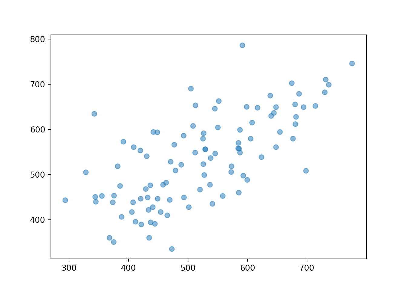
Notice the strong positive association; students who have high scores on one exam tend to have high scores on the other. We can simulate lots of values and construct a joint histogram.
(X & Y).sim(10000).plot('hist')## Error in py_call_impl(callable, dots$args, dots$keywords): ValueError: invalid literal for int() with base 10: ''plt.show() 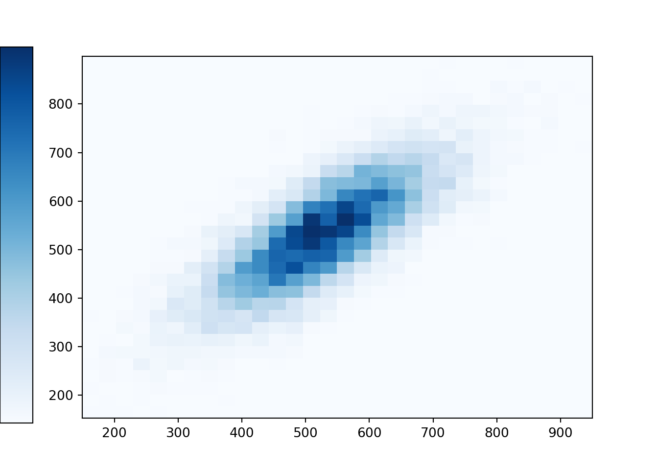
Recall that in some of the previous examples the shapes of one-dimensional histograms could be approximated with a smooth density curve. Similarly, a two-dimensional histogram can sometimes be approximated with a smooth density surface. As with histograms, the height of the density surface at a particular \((X, Y)\) pair of values can be represented by color intensity. A Normal distribution is a “bell-shaped curve”; a Bivariate Normal distribution is a “mound-shaped” curve — imagine a pile of sand. (Symbulate does not yet have the capability to display densities in a three-dimensional-like plot such as this plot.)
(X & Y).sim(10000).plot('density')
plt.show() 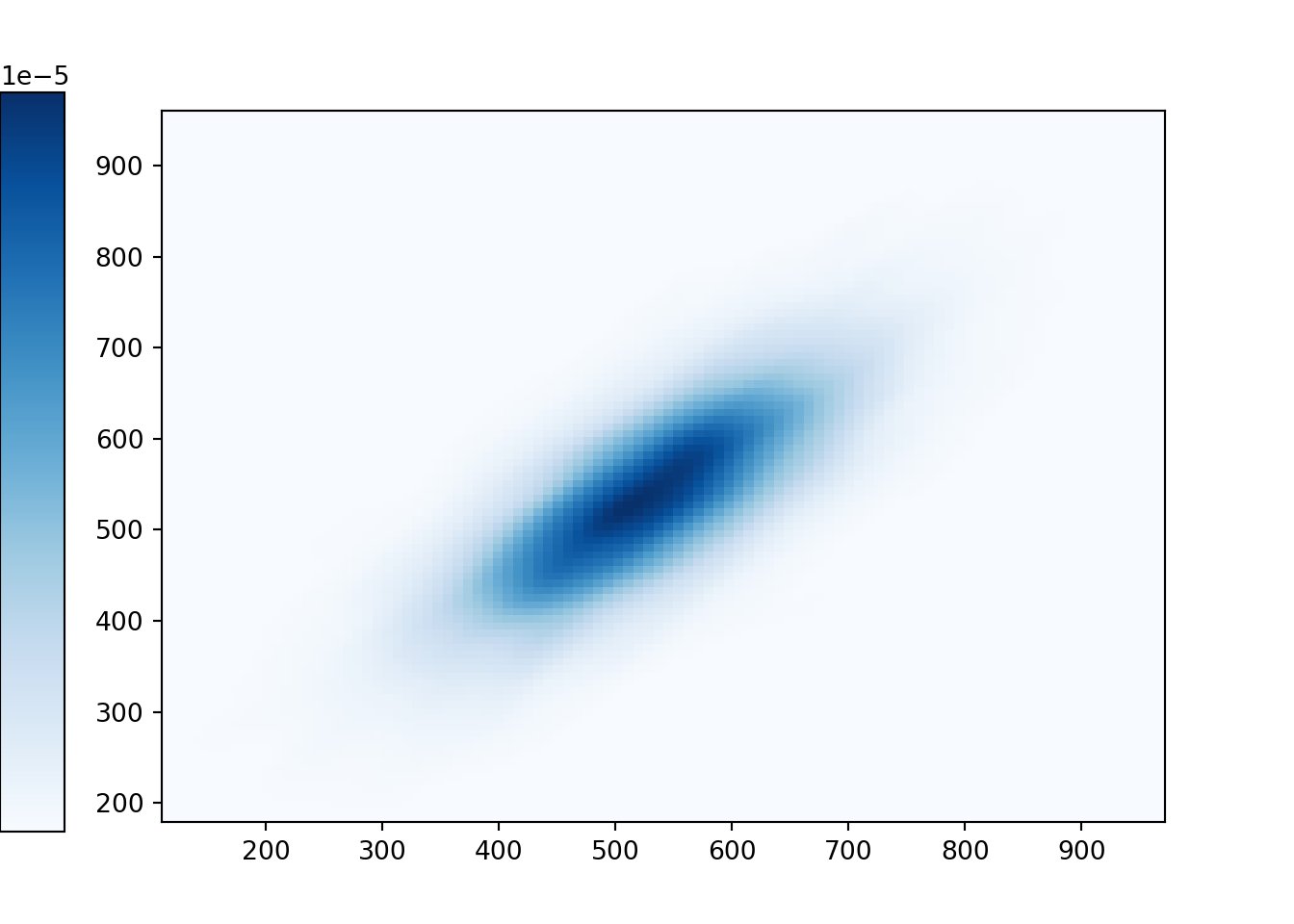
We can find marginal distributions by “aggregating/stacking/collapsing”. The SAT Math scores follow a Normal distribution with mean 527 and standard deviation 107, similarly for Reading.
X.sim(10000).plot()
plt.show()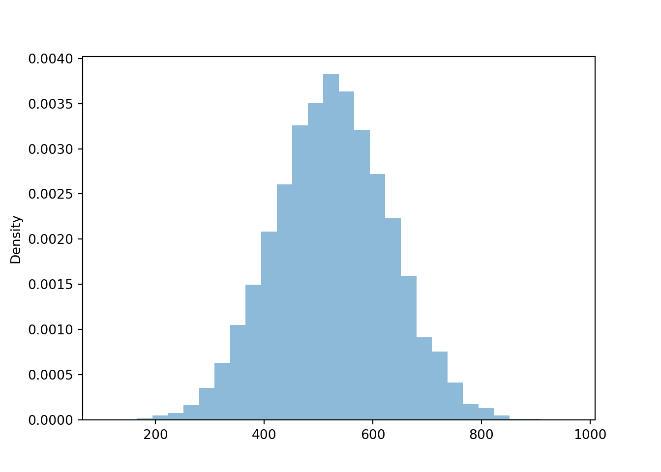
The value of correlation measures the strength of the association. For example, with a correlation of 0.4 the association would not be nearly as strong.
P = BivariateNormal(mean1 = 527, mean2 = 533, sd1 = 107, sd2 = 100, corr = 0.40)

X, Y = RV(P)

xy = (X & Y).sim(10000)

xy.plot('hist')
## Error in py_call_impl(callable, dots$args, dots$keywords): ValueError: invalid literal for int() with base 10: ''plt.show()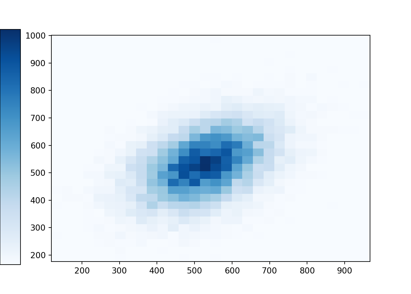
A negative correlation represents a negative association: large values of one variable tend to be associated with small values of the other. (This would not be realistic for SAT scores.)
P = BivariateNormal(mean1 = 527, mean2 = 533, sd1 = 107, sd2 = 100, corr = -0.77)

X, Y = RV(P)

xy = (X & Y).sim(10000)

xy.plot('hist')
## Error in py_call_impl(callable, dots$args, dots$keywords): ValueError: invalid literal for int() with base 10: ''plt.show()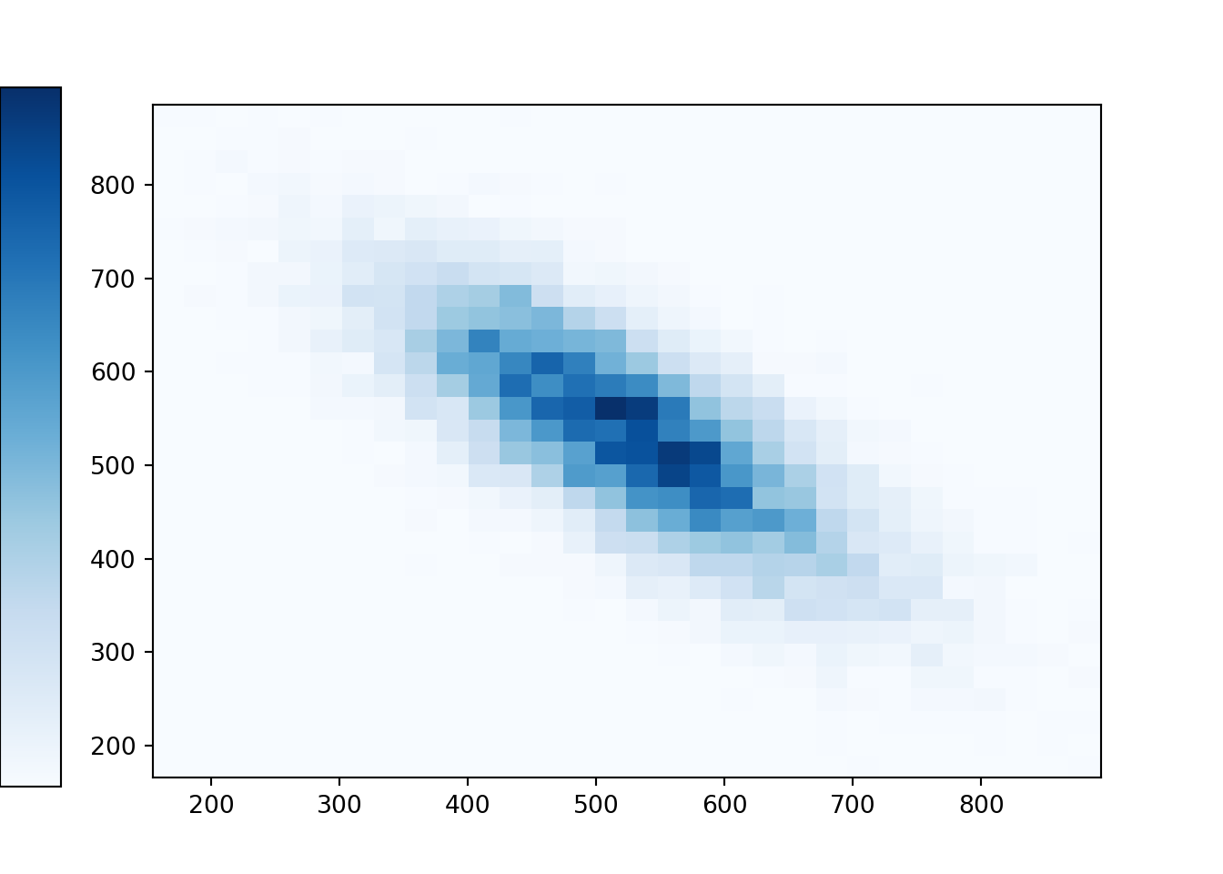
Note that in all of the above cases, the marginal distribution of Math scores is the same; likewise for Reading scores. But different correlations lead to different joint distributions. Remember: it is not possible to simulate \((X, Y)\) pairs simply from the marginal distributions.
Some lessons from this example.
- “Mound-shaped” Bivariate Normal distributions are the two-dimensional analogs of Normal distributions.
- Correlation is a measure of the strength of the association between two random variables.
- Remember: it is not possible to simulate \((X, Y)\) pairs simply from the marginal distributions.
We will see later that correlation measures the strength of a linear association: the degree to which pairs of values of the two random variables tend to follow a straight line.↩︎