4.8 Nonlinear transformations of random variables
The preceding section illustrated that a linear rescaling does not change the shape of a distribution, only the range of possible values. But what about a nonlinear transformation, like a logarithmic or square root transformation? In contrast to a linear rescaling, a nonlinear rescaling does not preserve relative interval length, so we might expect that a nonlinear rescaling can change the shape of a distribution. We’ll investigate by considering the Uniform(0, 1) spinner and a logarithmic85 transformation.
Let \(\textrm{P}\) be the probabilty space corresponding to the Uniform(0, 1) spinner and let \(U\) represent the result of a single spin. Attempting the transformation \(\log(U)\) leads to two minor technicalities.
- Since \(U\in[0, 1]\), \(\log(U)\le 0\). To obtain positive values we consider \(-\log(U)\), which takes values in \([0,\infty)\).
- Technically, applying \(-\log(u)\) to the values on the axis of the Uniform(0, 1) spinner, the resulting values would decrease from \(\infty\) to 0 clockwise. To make the values start at 0 and increase to \(\infty\) clockwise, we consider \(-\log(1-U)\). (We saw in the previous section the transformation \(u \to 1-u\) basically just changes direction from clockwise to counterclockwise.)
Therefore, it’s a little more convenient to consider the random variable \(X=-\log(1-U)\) which takes values in \([0,\infty)\). Remember: a transformation of a random variable is a random variable. Also, always be sure to identify the possible values that a random variable can take.
Before proceeding, try sketching a plot of the distribution of \(X\). (Just take a guess; you’ll get a chance to make a more educated sketch soon.)
The following code defines \(X\) and plots a few simulated values.
P = Uniform(0, 1)
U = RV(P)

X = -log(1 - U)

x = X.sim(100)

x.plot('rug')
plt.show()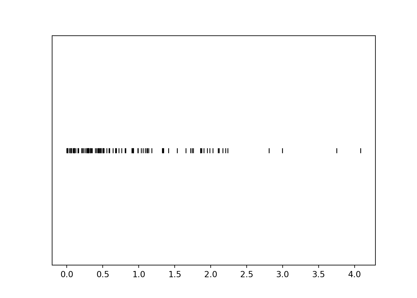
Notice that values near 0 occur with higher frequency than larger values. For example, there are many more simulated values of \(X\) that lie in the interval \([0, 1]\) than in the interval \([3, 4]\), even though these intervals both have length 1. Let’s see why this is happening before simulating many values.
Example 4.8 For each of the intervals in the table below find the probability that \(U\) lies in the interval, and identify the corresponding values of \(X\). (You should at least compute a few by hand to see what’s happening, but you can use software to fill in the rest.)
| Interval of U | Length of U interval | Probability | Interval of X | Length of X interval |
|---|---|---|---|---|
| (0, 0.1) | ||||
| (0.1, 0.2) | ||||
| (0.2, 0.3) | ||||
| (0.3, 0.4) | ||||
| (0.4, 0.5) | ||||
| (0.5, 0.6) | ||||
| (0.6, 0.7) | ||||
| (0.7, 0.8) | ||||
| (0.8, 0.9) | ||||
| (0.9, 1) |
Solution. to Example 4.8
Plug the endpoints into the conversion formula \(u\mapsto -\log(1-u)\) to find the corresponding \(X\) interval. For example, the \(U\) interval \((0.1, 0.2)\) corresponds to the \(X\) interval \((-\log(1-0.1), -\log(1-0.2))\). Since \(U\) has a Uniform(0, 1) distribution the probability is just the length of the \(U\) interval.
| Interval of U | Length of U interval | Probability | Interval of X | Length of X interval |
|---|---|---|---|---|
| (0, 0.1) | 0.1 | 0.1 | (0, 0.105) | 0.105 |
| (0.1, 0.2) | 0.1 | 0.1 | (0.105, 0.223) | 0.118 |
| (0.2, 0.3) | 0.1 | 0.1 | (0.223, 0.357) | 0.134 |
| (0.3, 0.4) | 0.1 | 0.1 | (0.357, 0.511) | 0.154 |
| (0.4, 0.5) | 0.1 | 0.1 | (0.511, 0.693) | 0.182 |
| (0.5, 0.6) | 0.1 | 0.1 | (0.693, 0.916) | 0.223 |
| (0.6, 0.7) | 0.1 | 0.1 | (0.916, 1.204) | 0.288 |
| (0.7, 0.8) | 0.1 | 0.1 | (1.204, 1.609) | 0.405 |
| (0.8, 0.9) | 0.1 | 0.1 | (1.609, 2.303) | 0.693 |
| (0.9, 1) | 0.1 | 0.1 | (2.303, Inf) | Inf |
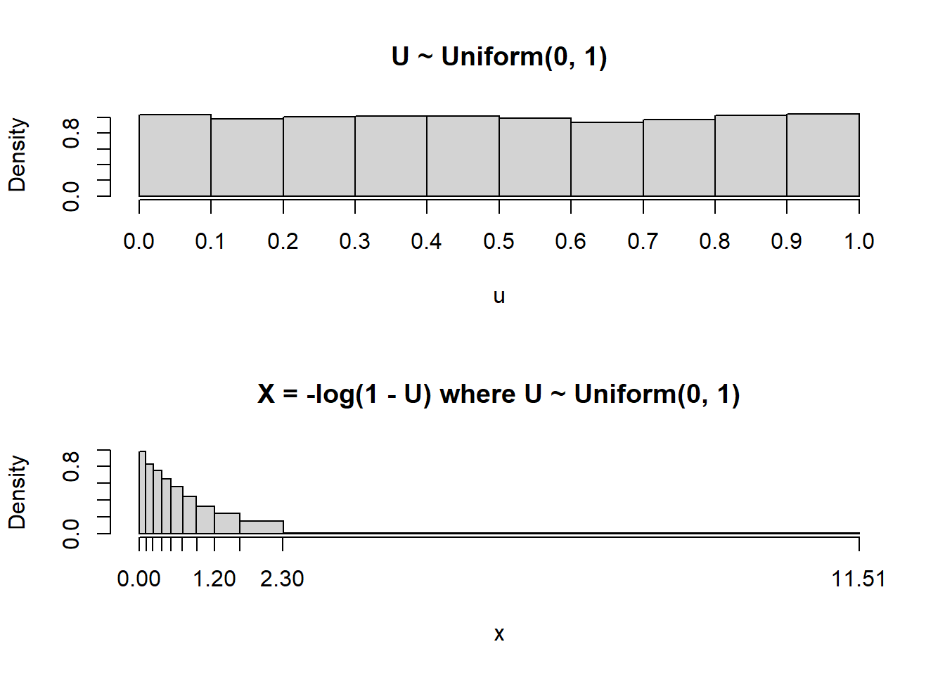
We see that the logarithmic transformation does not preserve relative interval length. Each of the original intervals of \(U\) values has the same length, but the nonlinear logarithmic transformation “stretches out” these intervals in different ways. The probability that \(U\) lies in each of these intervals is 0.1. As the transformation stretches the intervals, the 0.1 probability gets “spread” over different lengths of values. Since probability/relative frequency is represented by area in a histogram, if two regions of differing length have the same area, then they must have different heights. Thus the shape of the distribution of \(X\) will not be Uniform.
The following example provides a similar illustration, but from the reverse perspective.
Example 4.9 For each of the intervals of \(X\) values in the table below identify the corresponding values of \(U\), and then find the probability that \(X\) lies in the interval. (You should at least compute a few by hand to see what’s happening, but you can use software to fill in the rest.)
| Interval of X | Length of X interval | Probability | Interval of U | Length of U interval |
|---|---|---|---|---|
| (0, 0.5) | ||||
| (0.5, 1) | ||||
| (1, 1.5) | ||||
| (1.5, 2) | ||||
| (2, 2.5) | ||||
| (2.5, 3) | ||||
| (3, 3.5) | ||||
| (3.5, 4) | ||||
| (4, 4.5) | ||||
| (4.5, 5) |
Solution. to Example 4.9
The corresponding \(U\) intervals are obtained by applying the inverse transformation \(v\mapsto 1-e^{-v}\). For example, the \(X\) interval \((0.5, 1)\) corresponds to the \(U\) interval \((1-e^{-0.5}, 1-e^{-1})\).
| Interval of X | Length of X interval | Probability | Interval of U | Length of U interval |
|---|---|---|---|---|
| (0, 0.5) | 0.5 | 0.393 | (0, 0.393) | 0.393 |
| (0.5, 1) | 0.5 | 0.239 | (0.393, 0.632) | 0.239 |
| (1, 1.5) | 0.5 | 0.145 | (0.632, 0.777) | 0.145 |
| (1.5, 2) | 0.5 | 0.088 | (0.777, 0.865) | 0.088 |
| (2, 2.5) | 0.5 | 0.053 | (0.865, 0.918) | 0.053 |
| (2.5, 3) | 0.5 | 0.032 | (0.918, 0.95) | 0.032 |
| (3, 3.5) | 0.5 | 0.020 | (0.95, 0.97) | 0.020 |
| (3.5, 4) | 0.5 | 0.012 | (0.97, 0.982) | 0.012 |
| (4, 4.5) | 0.5 | 0.007 | (0.982, 0.989) | 0.007 |
| (4.5, 5) | 0.5 | 0.004 | (0.989, 0.993) | 0.004 |
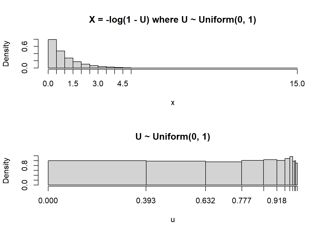
Since \(U\) has a Uniform(0, 1) distribution the probability is just the length of the \(U\) interval. Each of the \(X\) intervals has the same length but they correspond to intervals of differing length in the original \(U\) scale, and hence intervals of different probability.
Now we simulate many values of \(X\) and summarize the results in a histogram. But before proceeding, try again to sketch a plot of the distribution of \(X\). (You should be able to make a much more educated sketch now.)
X.sim(10000).plot()
Exponential(1).plot() # overlays the smooth curve
plt.show()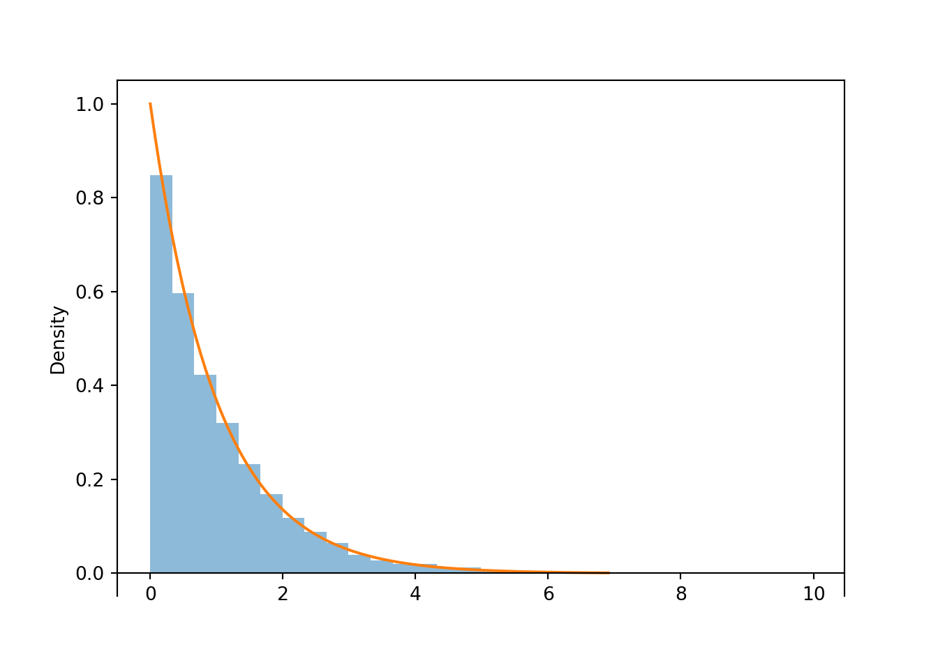
Figure 4.6: Histogram representing the approximate distribution of \(X=-\log(1-U)\), where \(U\) has a Uniform(0, 1) distribution. The smooth solid curve models the theoretical shape of the distribution of \(X\), known as the Exponential(1) distribution.
Notice that the shape of the histogram depicting the simulated values of \(X\) appears that it can be approximated by a smooth curve. This smooth curve is called the Exponential(1) density. We will see more properties of Exponential distributions later.
The following plots illustrate the results of Example 4.8 (plots on the left) and Example 4.9 (plots on the right), and give some insight into the shape of the distribution in Figure 4.6.
For a linear rescaling, we could just plug the mean of the original variable into the conversion formula to find the mean of the transformed variable. However, this will not work for nonlinear transformations.
(U & X).sim(10000).mean()## (0.4986607151628545, 0.9871809529241642)We see that the average value of \(U\) is about 0.5, the average value of \(X\) is about 1, and \(-\log(1 - 0.5) \neq 1\). The nonlinear “stretching” of the axis makes some value relatively larger and others relatively smaller than they were on the original scale, which influences the average. Remember, in general: Average of \(g(X)\) \(\neq\) \(g\)(Average of \(X\)).
What about a spinner which generates values according to the distribution in Figure 4.6? The “simulate from the probability space” method for simulating of \(X\) values entailed
- Spinning the Uniform(0, 1) spinner to get a value \(U\)
- Setting \(X=-\log(1-U)\)
These two steps can be combined by relabeling the values on the axis of the spinner according to the transformation \(u\mapsto -\log(1-u)\). For example, replace 0.1 by \(-\log(1-0.1)\approx 0.105\); replace 0.9 by \(-\log(1-0.9)\approx 2.30\). This transformation results in the spinner in Figure 4.7.
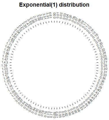
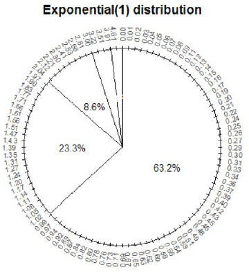
Figure 4.7: A spinner representing the distribution in Figure 4.6 (the “Exponential(1)” distribution.). The spinner is duplicated on the right; the highlighted sectors illustrate the non-linearity of axis values and how this translates to non-uniform probabilities.
Pay special attention to the values on the axis; they do not increase in equal increments. (As with the Uniform(0, 1) spinner, while only certain values are marked on the axis, we consider an idealized model in which any value in the continuous interval \([0, \infty)\) is a possible result of the spin.) The spinner on the right in Figure 4.7 is the same as the one on the left, with the intervals [0, 1], [1, 2], and [2, 3] highlighted with their respective probabilities. Putting a needle on this spinner that is “equally likely” to land anywhere on the axis, the needle will land in the interval [0, 1] with probability 0.632, in the interval [1, 2] with probability 0.233, etc. Therefore, values generated using this spinner, which represents the “Exponential(1)” distribution, will follow the pattern in Figure 4.6. Figure 4.8 illustrates this “simulate from a distribution” method; values of \(X\) are generated directly from an Exponential(1) distribution, rather than first generating \(U\) and then transforming.
X = RV(Exponential(1))

X.sim(10000).plot()
Exponential(1).plot()
plt.show()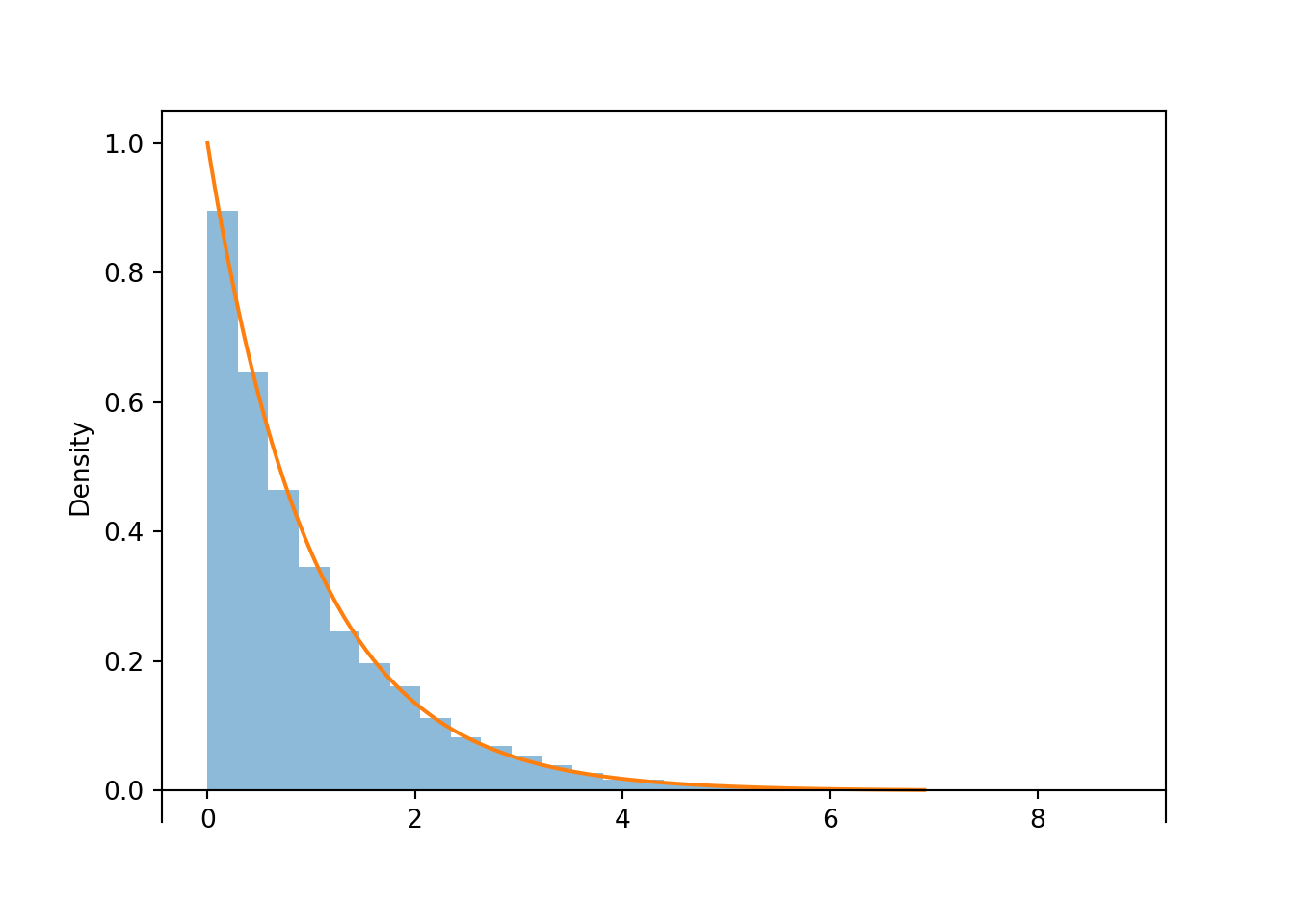
Figure 4.8: Simulated values from an Exponential(1) distribution, correspoding to the results of many spins of the spinner in Figure 4.6.
4.8.1 Summary
- Remember: a transformation of a random variable, both mathematically and in Symbulate.
- Be sure to always specify the possible values a random variable can take.
- A nonlinear transformation of a random variable changes the shape of its distribution (as well as the possible values).
- The shape of the histogram of simulated continuous values can be approximated by a smooth curve.
- Spinners can be used to generate values from non-uniform distributions by applying nonlinear transformations to values on the spinner axis.
- In general, Average of \(g(X)\) \(\neq\) \(g\)(Average of \(X\))
As in many other contexts and programming languages, in this text any reference to logarithms or \(\log\) refers to natural (base \(e\)) logarithms. In the instances we need to consider another base, we’ll make that explicit.↩︎