4.7 Transformations of random variables: Linear rescaling
A function of a random variable is a random variable: if \(X\) is a random variable and \(g\) is a function then \(Y=g(X)\) is a random variable. In general, the distribution of \(g(X)\) will have a different shape than the distribution of \(X\). The exception is when \(g\) is a linear rescaling.
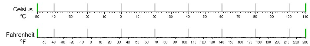
A linear rescaling is a transformation of the form \(g(u) = a +bu\), where \(a\) (intercept) and \(b\) (slope83) are constants. For example, converting temperature from Celsius to Fahrenheit using \(g(u) = 32 + 1.8u\) is a linear rescaling.
A linear rescaling “preserves relative interval length” in the following sense.
- If interval A and interval B have the same length in the original measurement units, then the rescaled intervals A and B will have the same length in the rescaled units. For example, [0, 10] and [10, 20] Celsius, both length 10 degrees Celsius, correspond to [32, 50] and [50, 68] Fahrenheit, both length 18 degrees Fahrenheit.
- If the ratio of the lengths of interval A and B is \(r\) in the original measurement units, then the ratio of the lengths in the rescaled units is also \(r\). For example, [10, 30] is twice as long as [0, 10] in Celsius; for the corresponding Fahrenheit intervals, [50, 86] is twice as long as [32, 50].
Think of a linear rescaling as just a relabeling of the variable axis.
Suppose that \(U\) has a Uniform(0, 1) distribution and define \(X = 200 + 600 U\). Then \(X\) is a linear rescaling of \(U\), and \(X\) takes values in the interval [200, 800]. We can define and simulate values of \(X\) in Symbulate. Before looking at the results, sketch a plot of the distribution of \(X\) and make an educated guess for its mean and standard deviation.
U = RV(Uniform(0, 1))

X = 200 + 600 * U

(U & X).sim(10)| Index | Result |
|---|---|
| 0 | (0.3750079992217965, 425.0047995330779) |
| 1 | (0.8902916681176966, 734.175000870618) |
| 2 | (0.19941328630280497, 319.647971781683) |
| 3 | (0.21577624704981235, 329.4657482298874) |
| 4 | (0.43146785270544497, 458.88071162326696) |
| 5 | (0.4169318285291006, 450.15909711746036) |
| 6 | (0.6596985317207639, 595.8191190324583) |
| 7 | (0.9627807371194141, 777.6684422716485) |
| 8 | (0.10264269383791114, 261.5856163027467) |
| ... | ... |
| 9 | (0.7043362221149847, 622.6017332689908) |
X.sim(10000).plot()
plt.show()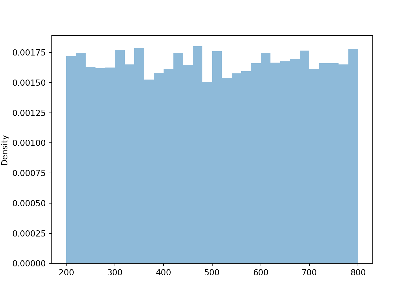
We see that \(X\) has a Uniform(200, 800) distribution. The linear rescaling changes the range of possible values, but the general shape of the distribution is still Uniform. We can see why by inspecting a few intervals on both the original and revised scale.
| Interval of \(U\) values | Probability that \(U\) lies in the interval | Interval of \(X\) values | Probability that \(X\) lies in the interval |
|---|---|---|---|
| (0.0, 0.1) | 0.1 | (200, 260) | \(\frac{60}{600}\) |
| (0.9, 1.0) | 0.1 | (740, 800) | \(\frac{60}{600}\) |
| (0.0, 0.2) | 0.2 | (200, 320) | \(\frac{120}{600}\) |
We have seen previously that the long run average value of \(U\) is 0.5, and of \(X\) is 500. These two values are related through the same formula mapping \(U\) to \(X\) values: \(500 = 200 + 600\times 0.5\).
The standard deviation of \(U\) is about 0.289, and of \(X\) is about 173.
print(U.sim(10000).sd(), X.sim(10000).sd())## 0.28931324273911185 172.3351978597985The standard deviation of \(X\) is 600 times the standard deviation of \(U\). Multiplying the \(U\) values by 600 rescales the distance between the values. Two values of \(U\) that are 0.1 units apart correspond to two values of \(X\) that are 60 units apart. However, adding the constant 200 to all values just shifts the distribution and does affect degree of variability.
In general, if \(U\) has a Uniform(0, 1) distribution then \(X = a + (b-a)U\) has a Uniform(\(a\), \(b\)) distribution. Therefore, we can essentially use the Uniform(0, 1) distribution to simulate values from any Uniform distribution.
Example 4.5 Let \(\textrm{P}\) be the probabilty space corresponding to the Uniform(0, 1) spinner and let \(U\) represent the result of a single spin. Define \(V=1-U\).
- Does \(V\) result from a linear rescaling of \(U\)?
- What are the possible values of \(V\)?
- Is \(V\) the same random variable as \(U\)?
- Find \(\textrm{P}(U \le 0.1)\) and \(\textrm{P}(V \le 0.1)\).
- Sketch a plot of what the histogram of many simulated values of \(V\) would look like.
- Does \(V\) have the same distribution as \(U\)?
Solution. to Example 4.5
Show/hide solution
- Yes, \(V\) result from the linear rescaling \(u\mapsto 1-u\) (intercept of 1 and slope of \(-1\).)
- \(V\) takes values in the interval [0,1]. Basically, this transformation just changes the direction of the spinner from clockwise to counterclockwise. The axis on the usual spinner has values \(u\) increasing clockwise from 0 to 1. Applying the transformation \(1-u\), the values would decrease clockwise from 1 to 0.
- No. \(V\) and \(U\) are different random variables. If the spin lands on \(\omega=0.1\), then \(U(\omega)=0.1\) but \(V(\omega)=0.9\). \(V\) and \(U\) return different values for the same outcome; they are measuring different things.
- \(\textrm{P}(U \le 0.1) = 0.1\) and \(\textrm{P}(V \le 0.1)=\textrm{P}(1-U \le 0.1) = \textrm{P}(U\ge 0.9) = 0.1\). Note, however, that these are different events: \(\{U \le 0.1\}=\{0 \le \omega \le 0.1\}\) while \(\{V \le 0.1\}=\{0.9 \le \omega \le 1\}\). But each is an interval of length 0.1 so they have the same probability according to the uniform probability measure.
- Since \(V\) is a linear rescaling of \(U\), the shape of the histogram of simulated values of \(V\) should be the same as that for \(U\). Also, the possible values of \(V\) are the same as those for \(U\). So the histograms should look identical (aside from natural simulation variability).
- Yes, \(V\) has the same distribution as \(U\). While for any single outcome (spin), the values of \(V\) and \(U\) will be different, over many repetitions (spins) the pattern of variation of the \(V\) values, as depicted in a histogram, will be identical to that of \(U\).
P = Uniform(0, 1)
U = RV(P)

V = 1 - U

V.sim(10000).plot()
plt.show()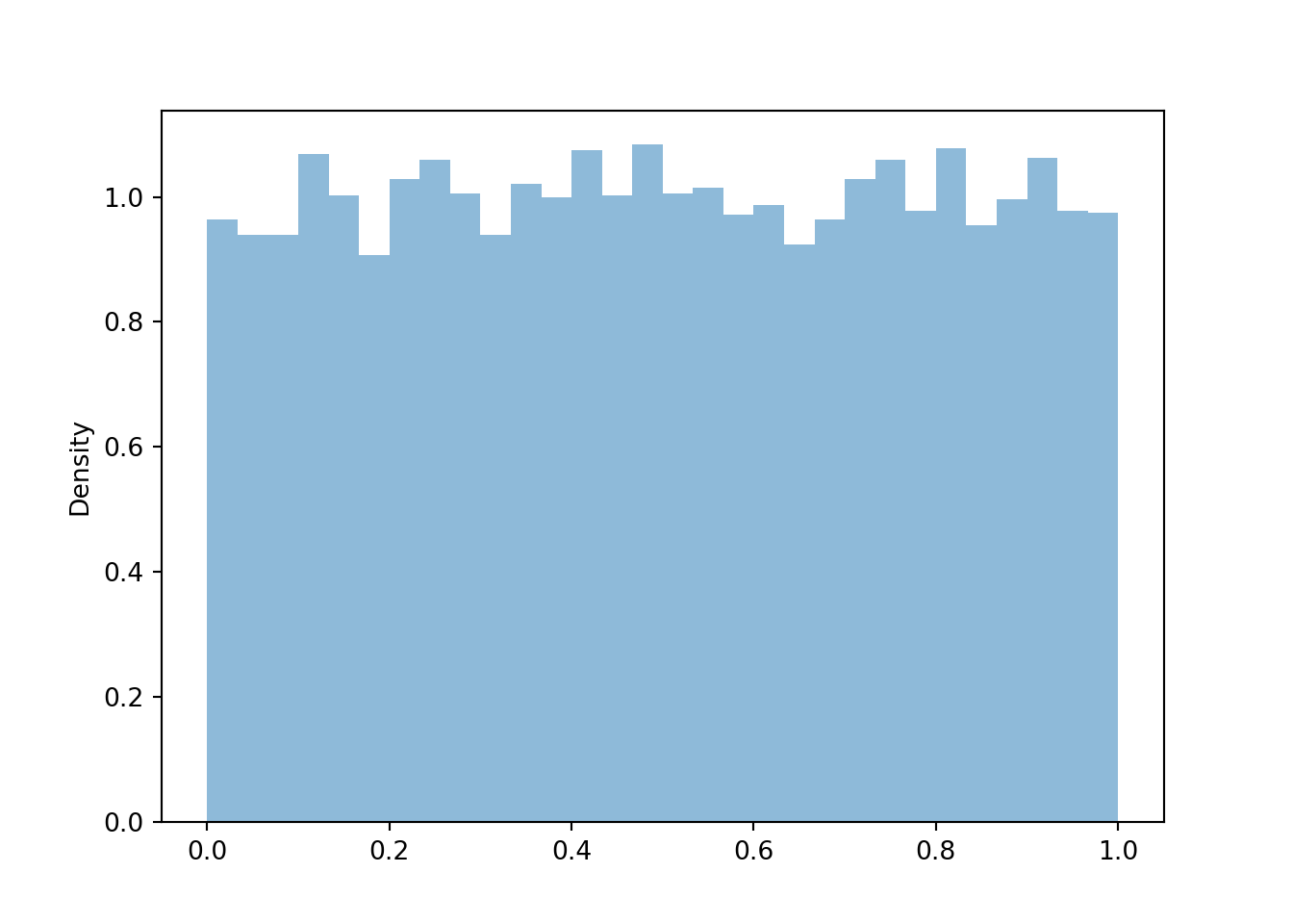
Let’s consider a non-uniform example. The spinner below represents a Normal distribution with mean 0 and standard deviation 1. Technically, with a Normal distribution any value in the interval \((-\infty, \infty)\) is possible. However, for a Normal(0, 1) distribution, the probability that a value lies outside the interval \((-3, 3)\) is small.
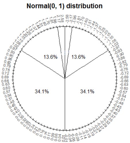
Let \(Z\) be a random variable with the Normal(0, 1) distribution. If we simulate many values of \(Z\):
- About half of the values would be below 0 and half above
- Because axis values near 0 are stretched out, simulated values near 0 would occur with higher frequency than those near -3 or 3.
- The shape of the distribution would be symmetric about 0 since the axis spacing of values below 0 mirrors that for values above 0. For example, about 34% of values would be between -1 and 0, and also 34% between 0 and 1.
- About 68% of values would be between -1 and 1.
- About 95% of values would be between -2 and 2.
Z = RV(Normal(0, 1))

z = Z.sim(10000)

z.plot()
Normal(0, 1).plot() # plot the density
plt.show()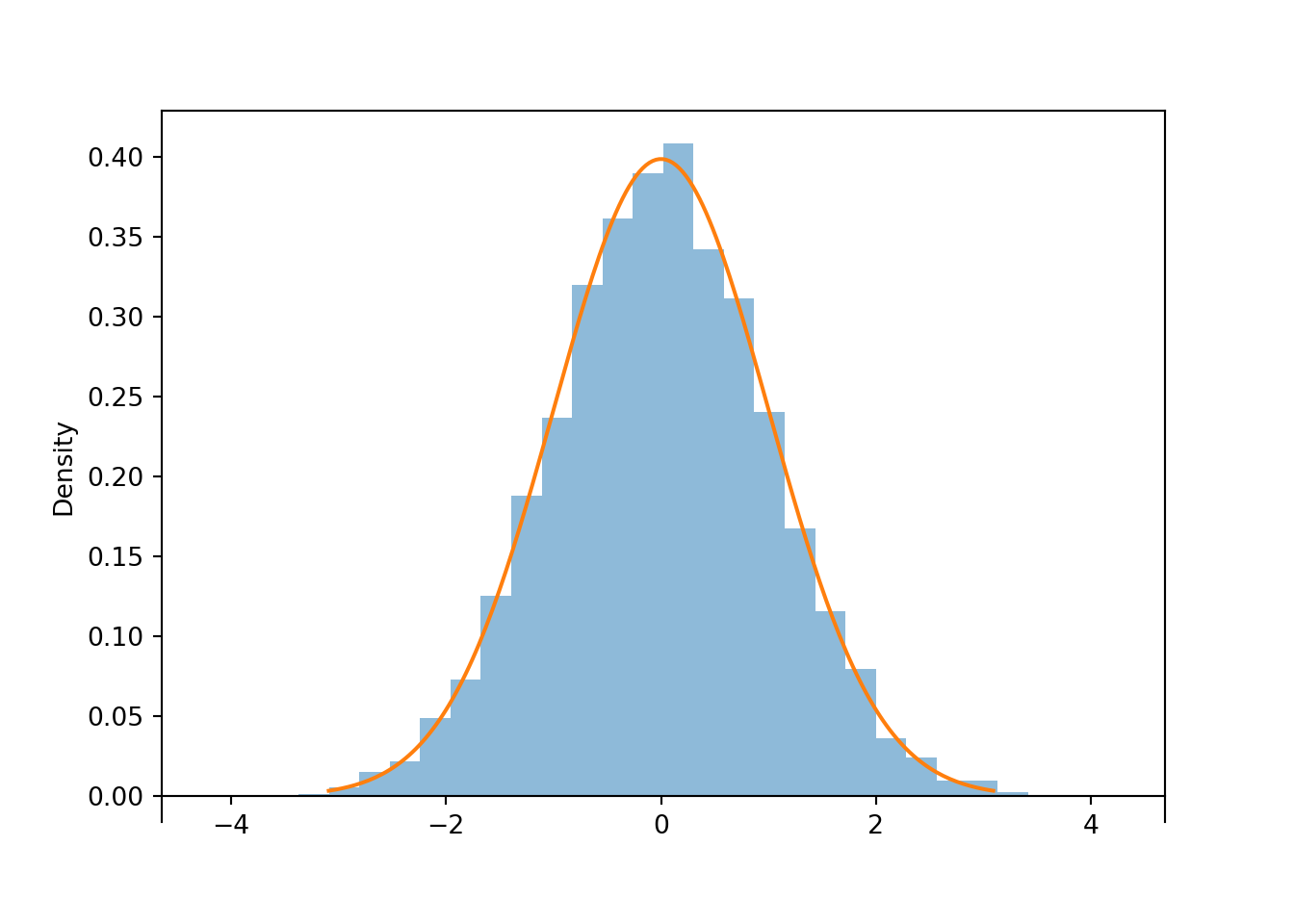
The long run average value of \(Z\) is 0 and the standard deviation is 1.
z.count_lt(-1) / z.count(), z.mean(), z.sd()## (0.1622, 0.002711924593052675, 1.009561063774299)Now consider the linear rescaling \(X=500 + 100 Z\). We see that \(X\) has a Normal(500, 100) distribution.
X = 500 + 100 * Z

(Z & X).sim(10)| Index | Result |
|---|---|
| 0 | (1.0029121298170771, 600.2912129817078) |
| 1 | (0.4081454217357649, 540.8145421735765) |
| 2 | (2.2470791127733416, 724.7079112773341) |
| 3 | (1.4115885507160892, 641.158855071609) |
| 4 | (-1.042249262323422, 395.7750737676578) |
| 5 | (0.5358927269442483, 553.5892726944248) |
| 6 | (-0.536915865248168, 446.3084134751832) |
| 7 | (-0.027615044699349604, 497.23849553006505) |
| 8 | (0.8755264332173788, 587.5526433217378) |
| ... | ... |
| 9 | (-0.397335627452405, 460.26643725475947) |
x = X.sim(10000)

x.plot()
Normal(500, 100).plot() # plot the density
plt.show()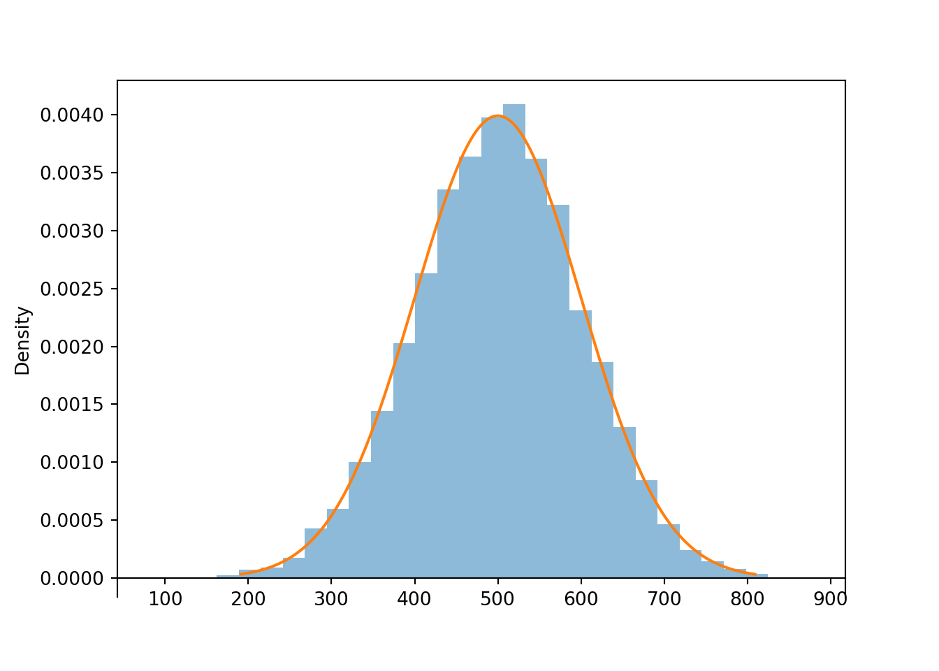
x.mean(), x.sd()## (501.22682029088094, 99.93430770040102)The linear rescaling changes the range of observed values; almost all of the values of \(Z\) lie in the interval \((-3, 3)\) while almost all of the values of \(X\) lie in the interval \((200, 800)\). However, the distribution of \(X\) still has the general Normal shape. The means are related by the conversion formula: \(500 = 500 + 100 \times 0\). Multiplying the values of \(Z\) by 100 rescales the distance between values; two values of \(Z\) that are 1 unit apart correspond to two values of \(X\) that are 100 units apart. However, adding the constant 500 to all the values just shifts the center of the distribution and does not affect variability. Therefore, the standard deviation of \(X\) is 100 times the standard deviation of \(Z\).
In general, if \(Z\) has a Normal(0, 1) distribution then \(X = \mu + \sigma Z\) has a Normal(\(\mu\), \(\sigma\)) distribution. Therefore, we can essentially use the Normal(0, 1) distribution to simulate values from any Normal distribution.
Example 4.6 Suppose that \(X\), the SAT Math score of a randomly selected student, follows a Normal(500, 100) distribution. Randomly select a student and let \(X\) be the student’s SAT Math score. Now have the selected student spin the Normal(0, 1) spinner. Let \(Z\) be the result of the spin and let \(Y=500 + 100 Z\).
- Is \(Y\) the same random variable as \(X\)?
- Does \(Y\) have the same distribution as \(X\)?
Solution. to Example 4.6
Show/hide solution
- No, these two random variables are measuring different things. One is measuring SAT Math score; one is measuring what comes out of a spinner. Taking the SAT and spinning a spinner are not the same thing.
- Yes, they do have the same distribution. Repeating the process of randomly selecting a student and measuring SAT Math score will yield values that follow a Normal(500, 100) distribution. Repeating the process of spinning the Normal(0, 1) spinner to get \(Z\) and then setting \(Y=500+100Z\) will also yield values that follow a Normal(500, 100) distribution. Even though \(X\) and \(Y\) are different random variables they follow the same long run pattern of variability.
Example 4.7 Let \(Z\) be a random variable with a Normal(0, 1) distribution. Consider \(-Z\).
- Donny Don’t says that the distribution of \(-Z\) will look like an “upside-down bell”. Is Donny correct? If not, explain why not and describe the distribution of \(-Z\).
- Donny Don’t says that the standard deviation of \(-Z\) is -1. Is Donny correct? If not, explain why not and determine the standard deviation of \(-Z\).
Solution. to Example 4.7
Show/hide solution
- Donny is confusing a random variable with its distribution. The values of the random variable are multiplied by -1, not the heights of the histogram. Multiplying values of \(Z\) by -1 rotates the “bell” about 0 horizontally (not vertically). Since the Normal(0, 1) distribution is symmetric about 0, the distribution of \(-Z\) is the same as the distribution of \(Z\), Normal(0, 1).
- Standard deviation cannot be negative. Standard deviation measures average distance of values from the mean. A \(Z\) value of 1 yields a \(-Z\) value of -1; in either case the value is 1 unit away from the mean. Multiplying a random variable by \(-1\) simply reflects the values horizontally about 0, but does not change distance from the mean84. In general, \(X\) and \(-X\) have the same standard deviation. In this example we can say more: \(Z\) and \(-Z\) have the same distribution so they must have the same standard deviation, 1.
4.7.1 Summary
- A linear rescaling is a transformation of the form \(g(u) = a + bu\).
- A linear rescaling of a random variable does not change the basic shape of its distribution, just the range of possible values.
- However, remember that the possible values are part of the distribution. So a linear rescaling does technically change the distribution, even if the basic shape is the same. (For example, Normal(500, 100) and Normal(0, 1) are two different distributions.)
- A linear rescaling transforms the mean in the same way the individual values are transformed.
- Adding a constant to a random variable does not affect its standard deviation.
- Multiplying a random variable by a constant multiplies its standard deviation by the absolute value of the constant.
- Whether in the short run or the long run, \[\begin{align*} \text{Average of $a+bX$} & = a+b(\text{Average of $X$})\\ \text{SD of $a+bX$} & = |b|(\text{SD of $X$})\\ \text{Variance of $a+bX$} & = b^2(\text{Variance of $X$}) \end{align*}\]
- If \(U\) has a Uniform(0, 1) distribution then \(X = a + (b-a)U\) has a Uniform(\(a\), \(b\)) distribution.
- If \(Z\) has a Normal(0, 1) distribution then \(X = \mu + \sigma Z\) has a Normal(\(\mu\), \(\sigma\)) distribution.
- Remember, do NOT confuse a random variable with its distribution.
- The random variable is the numerical quantity being measured
- The distribution is the long run pattern of variation of many observed values of the random variable
You might be familiar with “\(mx+b\)” where \(b\) denotes the intercept. In Statistics, \(b\) is often used to denote slope. For example, in R
abline(a = 32, b = 1.8)draws a line with intercept 32 and slope 1.8.↩︎If the mean were not 0, multiplying a random variable by \(-1\) reflects the mean about 0 too, and distances from the mean are unaffected. For example, suppose \(X\) has mean 1 so a value of 5 is 4 units away from the mean of 1. Then \(-X\) has mean -1; a value of \(X\) of 5 yields a value of \(-X\) of -5, which is 4 units away from the mean of -1.↩︎