7.2 Properties of conditional probability
The impeachment problem in the previous section illustrated a few concepts that we will explore in more detail in the next few sections.
7.2.1 Multiplication rule
Multiplication rule: the probability that two events both occur is \[\begin{aligned} \textrm{P}(A \cap B) & = \textrm{P}(A|B)\textrm{P}(B)\\ & = \textrm{P}(B|A)\textrm{P}(A)\end{aligned}\]
The multiplication rule says that you should think “multiply” when you see “and”. However, be careful about what you are multiplying: to find a joint probability you need an unconditional and an appropriate conditional probability. You can condition either on \(A\) or on \(B\), provided you have the appropriate marginal probability; often, conditioning one way is easier than the other. Be careful: the multiplication rule does not say that \(\textrm{P}(A\cap B)\) is the same as \(\textrm{P}(A)\textrm{P}(B)\).
Generically, the multiplication rule says \[ \text{joint} = \text{conditional}\times\text{marginal} \]
For example:
- 31% of Americans are Democrats
- 83.9% of Democrats support impeachment
- So 26% of Americans are Democrats who support impeachment, \(0.26 = 0.31\times 0.839\).
\[ \frac{\text{Democrats who support impeachment}}{\text{Americans}} = \left(\frac{\text{Democrats}}{\text{Americans}}\right)\left(\frac{\text{Democrats who support impeachment}}{\text{Democrats}}\right) \]
The multiplication rule extends naturally to more than two events. \[ \textrm{P}(A_1\cap A_2 \cap \cdots \cap A_{k}) = \textrm{P}(A_1)\textrm{P}(A_2|A_1)\textrm{P}(A_3|A_1\cap A_2) \times \cdots \times \textrm{P}(A_k|A_1 \cap A_2 \cap \cdots \cap A_{k-1}) \]
The multiplication rule is useful for computing probabilities for a random phenomenon that can be broken down into component “stages”.
Example 7.6 The birthday problem concerns the probability that at least two people in a group of \(n\) people have the same birthday123. In particular, how large does \(n\) need to be in order for this probability to be larger than 0.5? Ignore multiple births and February 29 and assume that the other 365 days are all equally likely124.
- Explain how, in principle, you could perform a tactile simulation to estimate the probability that at least two people have the same birthday when \(n=30\).
- For \(n=30\), find the probability that none of the people have the same birthday.
- For \(n=30\), find the probability that at least two people have the same birthday.
- Write a clearly worded sentence interpreting the probability in the previous part as a long run relative frequency.
- When \(n=30\), how much more likely than not is it for at least two people to have the same birthday?
- Provide an expression of the probability for a general \(n\) and find the smallest value of \(n\) for which the probability is over 0.5. (You can just try different values of \(n\).)
- When \(n=100\) the probability is about 0.9999997. If you are in a group of 100 people and no one shares your birthday, should you be surprised?
Solution. to Example 7.6
Show/hide solution
Here is one way.
- Get 365 cards and label each one with a distinct birthday.
- Shuffle the cards and select 30 with replacement.
- Record whether or not you selected at least one card more than once. This corresponds to at least two people sharing a birthday.
- Repeat many times; each repetition consists of a selecting a sample of 30 cards with replacement.
- Find the proportion of repetitions on which at least two people had the same birthday to approximate the probability.
In the simulation below, the random variable \(X\) measures the number of distinct birthdays among the 30 people. So if no one shares a birthday then \(X=30\), if exactly two people share a brithday then \(X=29\), and so on.
Imagine lining the 30 people up in some order. Let \(A_2\) be the event that the first two people have different birthdays, \(A_3\) be the event that the first three people have different birthdays, and so on, until \(A_{30}\), the event that all 30 people have different birthdays. Notice \(A_{30}\subseteq A_{29} \subseteq \cdots \subseteq A_3 \subseteq A_2\), so \(\textrm{P}(A_{30}) = \textrm{P}(A_2 \cap A_3 \cap \cdots \cap A_{30})\).
The first person’s birthday can be any one of 365 days. In order for the second person’s birthday to be different, it needs to be on one of the remaining 364 days. So the probability that the second person’s birthday is different from the first is \(\textrm{P}(A_2)=\frac{364}{365}\).
Now if the first two people have different birthdays, in order for the third person’s birthday to be different it must be on one of the remaining 363 days. So \(\textrm{P}(A_3|A_2) = \frac{363}{365}\). Notice that this is a conditional probability. (If the first two people had the same birthday, then the probability that the third person’s birthday is different would be \(\frac{364}{365}\).)
If the first three people have different birthdays, in order for the fourth person’s birthday to be different it must be on one of the remaining 362 days. So \(\textrm{P}(A_4|A_2\cap A_3) = \frac{362}{365}\).
And so on. If the first 29 people have different birthdays, in order for the 30th person’s birthday to be different it must be on one of the remaining 365-29=336 days. Then using the multiplication rule
\[\begin{align*} \textrm{P}(A_{30}) & = \textrm{P}(A_{2}\cap A_3 \cap \cdots \cap A_{30})\\ & = \textrm{P}(A_2)\textrm{P}(A_3|A_2)\textrm{P}(A_4|A_2\cap A_3)\textrm{P}(A_5|A_2\cap A_3 \cap A_4)\cdots \textrm{P}(A_{30}|A_2\cap \cdots \cap A_{29})\\ & = \left(\frac{364}{365}\right)\left(\frac{363}{365}\right)\left(\frac{362}{365}\right)\left(\frac{361}{365}\right)\cdots \left(\frac{365-30 + 1}{365}\right)\approx 0.294 \end{align*}\]
By the complement rule, the probability that at least two people have the same birthday is \(1-0.294=0.706\), since either (1) none of the people have the same birthday, or (2) at least two of the people have the same birthday.
In about 70% of groups of 30 people at least two people in the group will have the same birthday. For example, if Cal Poly classes all have 30 students, then in about 70% of your classes at least two people in the class will share a birthday.
\(0.706 / 0.294 = 2.4.\) In a group of \(n=30\) people it is about 2.4 times more likely to have at least two people with the same birthday than not.
For a general \(n\), the probability that at least two people have the same birthday is \[ 1 - \prod_{k=1}^{n}\left(\frac{365-k+1}{365}\right) \] See the plot below, which plots this probability as a function of \(n\). When \(n=23\) this probability is 0.507.
Maybe, but not because of the 0.999997. That probability is the probability that at least two people in the group of 100 share a birthday. It is NOT the probability that someone shares YOUR birthday. (We will see later how to compute the probability that no one shares your birthday as \((364/365)^{100}= 0.76\). So it’s not very surprising that no one shares your birthday.)
def count_distinct_values(list):
    return len(set(list))

n = 30
P = BoxModel(list(range(365)), size = n, replace = True)
X = RV(P, count_distinct_values)

x = X.sim(10000)

x.plot()
plt.show()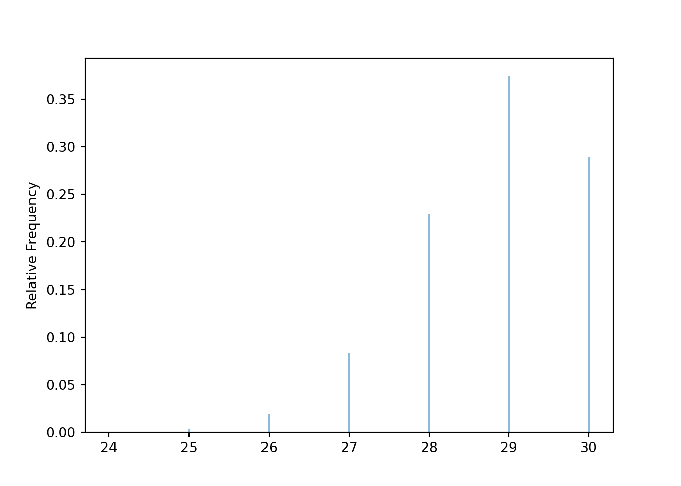
Figure 7.3: Simulation of the birthday problem for \(n=30\). The plot displays the simulated distribution of the number of distinct birthdays among the 30 people. There are no birthday matches only when there are 30 distinct birthdays among the 30 people, which happens with probability about 0.3.
x.count_lt(n) / 10000## 0.7111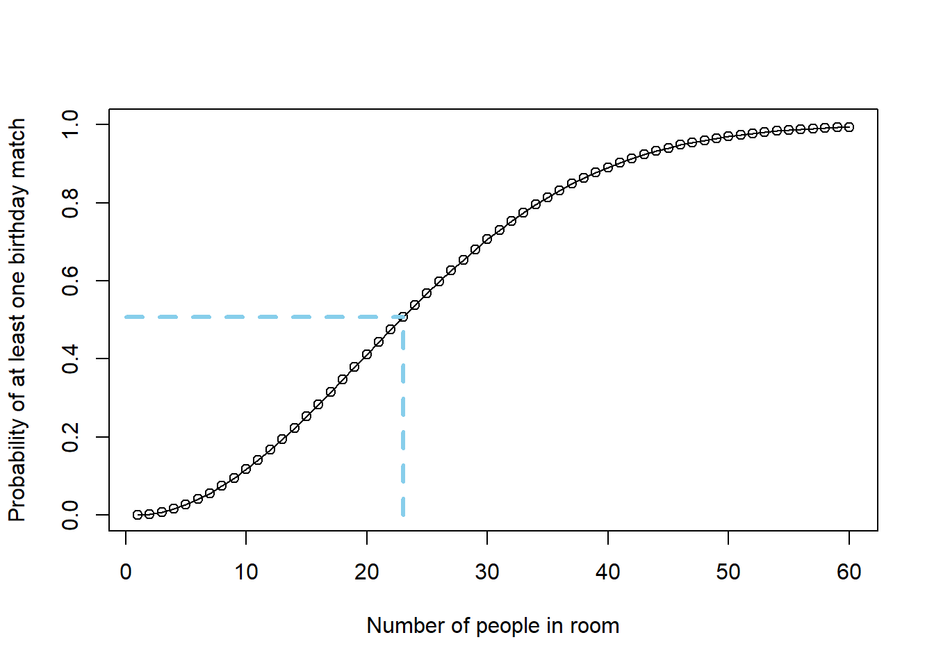
Figure 7.4: Probability of at least one birthday match as a function of the number of people in the room. For 23 people, the probability of at least one birthday match is 0.507.
7.2.2 Law of total probability
The “overall” unconditional probability \(\textrm{P}(A)\) can be thought of as a weighted average of the “case-by-case” conditional probabilities \(\textrm{P}(A|B)\) and \(\textrm{P}(A|B^c)\), where the weights are determined by the likelihood of each case, \(\textrm{P}(B)\) versus \(\textrm{P}(B^c)\). \[ \textrm{P}(A) = \textrm{P}(A|B)\textrm{P}(B) + \textrm{P}(A|B^c)\textrm{P}(B^c) \] This is an example of the law of total probability, which applies even when there are more than two cases.
Law of total probability. If \(C_1,\ldots, C_k\) are disjoint with \(C_1\cup \cdots \cup C_k=\Omega\), then \[\begin{align*} \textrm{P}(A) & = \sum_{i=1}^k \textrm{P}(A \cap C_i)\\ & = \sum_{i=1}^k \textrm{P}(A|C_i) \textrm{P}(C_i) \end{align*}\]
The events \(C_1, \ldots, C_k\), which represent the “cases”, form a partition of the sample space; each outcome \(\omega\in\Omega\) lies in exactly one of the \(C_i\). The law of total probability says that we can interpret the unconditional probability \(\textrm{P}(A)\) as a probability-weighted average of the case-by-case conditional probabilities \(\textrm{P}(A|C_i)\) where the weights \(\textrm{P}(C_i)\) represent the probability of encountering each case.
For an illustration of the law of total probability, consider the single bar to the right of the plot on the left in Figure 7.2 which displays the marginal probability of supporting/not supporting impeachment. The height within this bar is the weighted average of the heights within the other bars, with the weights given by the widths of the other bars.
The plot on the right in 7.2 represents conditioning on support of impeachment. Now the widths of the vertical bars represent the distribution of supporting/not supporting impeachment, the heights within the bars represent conditional probabilities for party affiliation given support status, and the single bar to the right represents the marginal distribution of party affiliation. Now we can see that the marginal probabilities for part affiliation are the weighted averages of the respective conditional probabilities given support status.
Conditioning and using the law of probability is an effective strategy in solving many problems. For example, when a problem involves iterations or steps it is often useful to condition on the result of the first step.
Example 7.7 You and your friend are playing the “lookaway challenge”.
In the first round, you point in one of four directions: up, down, left or right. At the exact same time, your friend also looks in one of those four directions. If your friend looks in the same direction you’re pointing, you win! Otherwise, you switch roles as the game continues to the next round — now your friend points in a direction and you try to look away. As long as no one wins, you keep switching off who points and who looks.
Suppose that each player is equally likely to point/look in each of the four directions, independently from round to round. What is the probability that you win the game?
- Why might you expect the probability to not be equal to 0.5?
- What is the probability that you win in the first round?
- If \(p\) denotes the probability that the player who goes first (you) wins, what is the probability that the other player wins?
- Condition on the result of the first round and set up an equation to solve for \(p\).
Solution. to Example 7.7
Show/hide solution
- The player who plays first has the advantage of going first; that player can win the game in the first round, but cannot lose the game in the first round. So we might expect the player who goes first to be more likely to win than the other player.
- 1/4. If we represent an outcome in the first round as a pair (point, look) then there are 16 possible equally likely outcomes, of which 4 represent pointing and looking in the same direction. Alternatively, whichever direction you point, the probability that your friend looks in the same direction is 1/4.
- \(1-p\), since the game keeps going until someone wins.
- Here is where we use conditioning and the law of total probability. Let \(A\) be the event that you win the game, and \(B\) be the event that you win in the first round. By the law of total probability \[ \textrm{P}(A) = \textrm{P}(A|B)\textrm{P}(B) + \textrm{P}(A|B^c)\textrm{P}(B^c) \] Now \(\textrm{P}(A)=p\), \(\textrm{P}(B)=1/4\), \(\textrm{P}(B^c)=3/4\), and \(\textrm{P}(A|B)=1\) since if you win in the first round then you win the game. Now consider \(\textrm{P}(A|B^c)\). If you don’t win in the first round, it is like the game starts over with the other playing going first. In this scenario, you play the role of the player who does not go first, and we saw above that the probability that the player who does not go first wins is \(1-p\). That is, \(\textrm{P}(A|B^c) = 1-p\). Therefore \[ p = (1)(1/4)+ (1-p)(3/4) \] Solve to find \(p=4/7\approx 0.57\).
The following is one way to code the lookaway challenge. In each round an outcome is a (point, look) pair, coded with a BoxModel with size=2 (and choices labeled 1, 2, 3, 4). The ** inf assumes the rounds continue indefinitely, so the outcome of a game is a sequence of (point, look) pairs for each round. The random variable \(X\) counts the number of rounds until there is a winner, which occurs in the first round that point = look. The player who goes first wins the game if the game ends in an odd number of rounds, so to estimate the probability that the player who goes first wins we find the proportion of repetitions in which \(X\) is an odd number.
def is_odd(x):
    return (x % 2) == 1

def count_rounds(sequence):
    for r, pair in enumerate(sequence):
        if pair[0] == pair[1]:
            return r + 1 # +1 for 0 indexing

P = BoxModel([1, 2, 3, 4], size = 2) ** inf
X = RV(P, count_rounds)
x = X.sim(10000)


x.plot()
plt.show()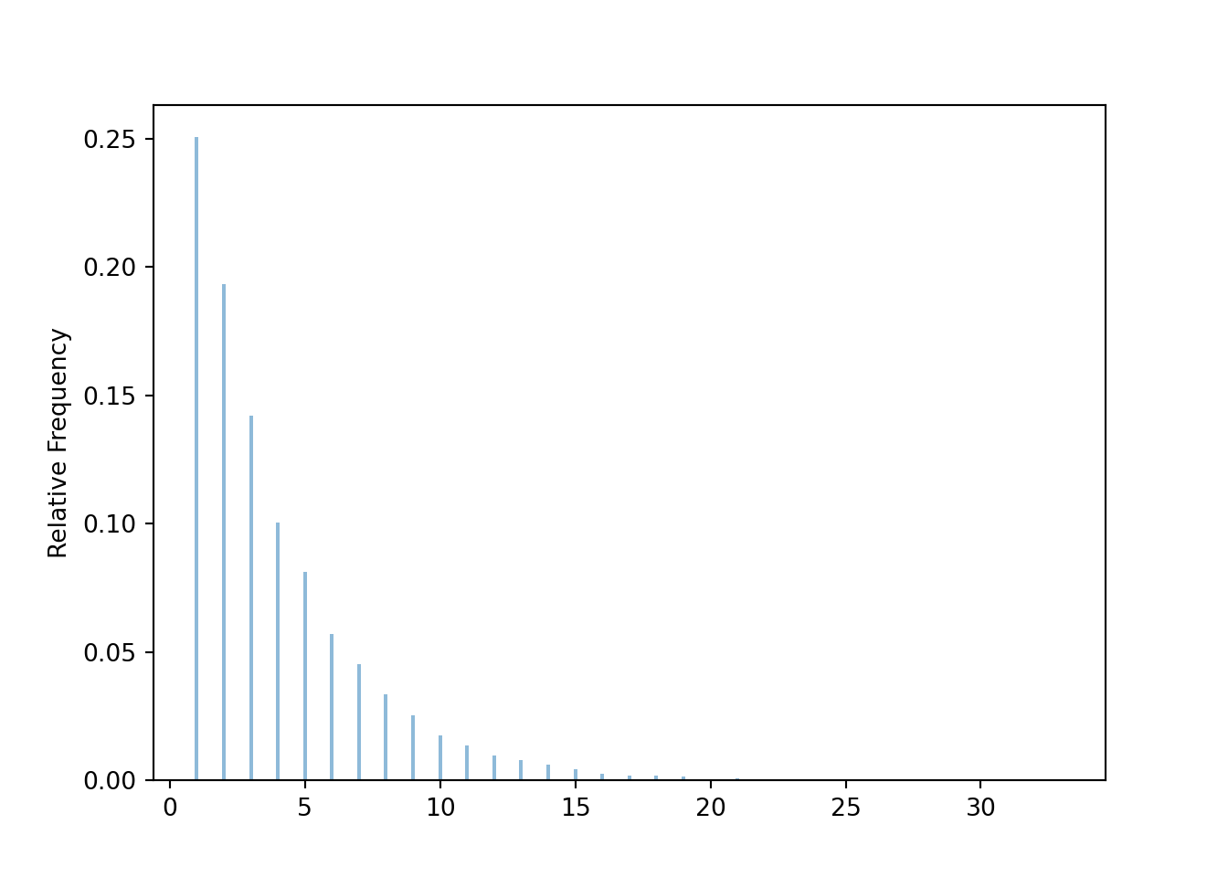
print(x.count(is_odd) / 10000)## 0.57617.2.3 Bayes rule
Bayes’ rule specifies how a prior probability \(\textrm{P}(B)\) is updated in response to information that event \(B\) has occurred to obtain the posterior probability \(\textrm{P}(B|A)\). \[ \textrm{P}(B|A) = \textrm{P}(B)\left(\frac{\textrm{P}(A|B)}{\textrm{P}(A)}\right) \]
Bayes’ rule is often used in conjunction with the law of total probability. If \(C_1,\ldots, C_k\) are disjoint with \(C_1\cup \cdots \cup C_k=\Omega\), then for any \(j\)
\[\begin{align*} \textrm{P}(C_j|A) & = \frac{\textrm{P}(A|C_j)\textrm{P}(C_j)}{\sum_{j=1}^k \textrm{P}(A|C_i) \textrm{P}(C_i)} \end{align*}\]
Each of the \(C_j\) represents a different “case” or “hypothesis”, while \(A\) represents “evidence” or “data”. So Bayes’ rule gives a way of updating \(\textrm{P}(C_j)\), the prior probability of hypothesis \(C_j\), in light of evidence \(A\) to obtain the posterior probability \(\textrm{P}(C_j|A)\).
Example 7.8 A woman’s chances of giving birth to a child with Down syndrome increase with age. The CDC estimates125 that a woman in her mid-to-late 30s has a risk of conceiving a child with Down syndrome of about 1 in 250. A nuchal translucency (NT) scan, which involves a blood draw from the mother and an ultrasound, is often performed around the 13th week of pregnancy to test for the presence of Down syndrome (among other things). If the baby has Down syndrome, the probability that the test is positive is about 0.9. However, when the baby does not have Down syndrome, there is still a probability that the test returns a (false) positive of about126 0.05. Suppose that the NT test for a pregnant woman in her mid-to-late 30s comes back positive for Down syndrome. What is the probability that the baby actually has Down syndrome?
- Before proceeding, make a guess for the probability in question. \[ \text{0-20\%} \qquad \text{20-40\%} \qquad \text{40-60\%} \qquad \text{60-80\%} \qquad \text{80-100\%} \]
- Donny Don’t says: 0.90 and 0.05 should add up to 1, so there must be a typo in the problem. Do you agree?
- Let \(D\) be the event that the baby has Down Syndrome, and let \(T\) be the event that the test is positive. Represent the probabilities provided using proper notation. Also, denote the probability that we are trying to find.
- Considering a hypothetical population of babies (of pregnant women in this demographic), express the probabilities as percents in context.
- Construct a hypothetical two-way table of counts.
- Use the table to find the probability in question.
- Using the probabilities provided in the setup, and without using the two-way table, find the probability that the test is positive.
- Using the probabilities provided in the setup, and without using the two-way table, find the probability that the baby actually has Down syndrome given that the test is positive.
- The probability in the previous part might seem very low to you. Explain why the probability is so low.
- Compare the probability of having Down Syndrome before and after the positive test. How much more likely is a baby who tests positive to have Down Syndrome than a baby for whom no information about the test is available?
Solution. to Example 7.8
Show/hide solution
We don’t know what you guessed, but from experience many people guess 80-100%. Afterall, the test is correct for most of the babies who have Down Syndrome, and also correct for the most of the babies who do not have Down Syndrome, so it seems like the test is correct most of the time. But this argument ignores one important piece of information that has a huge impact on the results: most babies do not have Down Syndrome.
No, these probabilities apply to different groups: 0.9 to babies with Down Syndrome, and 0.05 to babies without Down Syndrome. Donny is using the complement rule incorrectly. For example, if 0.9 is the probability that a baby with Down Syndrome tests positive, then 0.1 is the probability that a baby with Down Syndrome does not test positive; both probabilities apply to babies with Down Syndrome, and each baby with Down Syndrome either tests positive or not.
If \(D\) is the event that the baby has Down Syndrome, and \(T\) is the event that the test is positive, then we are given
- \(\textrm{P}(D) = 1/250 = 0.004\)
- \(\textrm{P}(T|D) = 0.9\)
- \(\textrm{P}(T|D^c) = 0.05\)
- We want to find: \(\textrm{P}(D|T)\).
Considering a hypothetical population of babies (of pregnant women in this demographic):
- 0.4% of babies have Down Syndrome
- 90% of babies with Down Syndrome test positive
- 5% of babies without Down Syndrome test positive
- We want to find the percentage of babies who test positive that have Down Syndrome.
Assuming 10000 babies (of pregnant women in this demographic)
Has Down Syndrome Does Not have Down Sydrome Total Tests positive 36 498 534 Not test positive 4 9462 9466 Total 40 9960 10000 Among the 534 babies who test positive, 36 have Down Syndrome, so the probability that a baby who tests positive has Down Syndrome is 36/534 = 0.067.
Use the law of total probability: the probability of testing positive is the weighted average of 0.9 and 0.05; 0.05 gets much more weight because there are many more babies without Down Syndrome \[ \textrm{P}(T) = \textrm{P}(T|D)\textrm{P}(D) + \textrm{P}(T|D^c)\textrm{P}(D^c) = 0.9(0.004) + 0.05(0.996) = 0.0534 \]
Use Bayes’ rule \[ \textrm{P}(D|T) = \frac{\textrm{P}(T|D)\textrm{P}(D)}{\textrm{P}(T)} = \frac{0.9(0.004)}{0.0534} = 0.067. \]
The result says that only 6.7% of babies who test positive actually have Down Syndrome. It is true that the test is correct for most babies with Down Syndrome (36 out of 40) and incorrect only for a small proportion of babies without Down Syndrome (498 out of 9960). But since so few babies have Down Syndrome, the sheer number of false positives (498) swamps the number of true positives (36).
Prior to observing the test result, the prior probability that a baby has Down Syndrome is 0.004. The posterior probability that a baby has Down Syndrome given a positive test result is 0.067. A baby who tests positive is about 17 times (0.067/0.004) more likely to have Down Syndrome than a baby for whom the test result is not known. So while 0.067 is still small in absolute terms, the posterior probability is much larger relative to the prior probability.
Remember, the conditional probability of \(A\) given \(B\), \(\textrm{P}(A|B)\), is not the same as the conditional probability of \(B\) given \(A\), \(\textrm{P}(B|A)\), and they can be vastly different. Remember to ask “percentage of what”? For example, the percentage of babies who have Down syndrome that test positive is a very different quantity than the percentage of babies who test positive that have Down syndrome.
Conditional probabilities (\(\textrm{P}(D|T)\)) can be highly influenced by the original unconditional probabilities (\(\textrm{P}(D)\)) of the events, sometimes called the base rates. Don’t neglect the base rates when evaluating probabilities. The example illustrates that when the base rate for a condition is very low and the test for the condition is less than perfect there will be a relatively high probability that a positive test is a false positive.
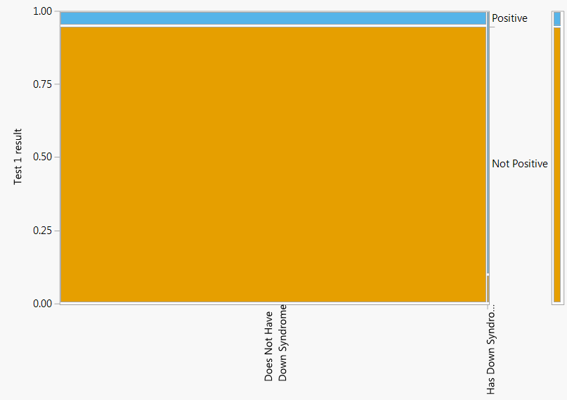 7.8. The plot on the left represents conditioning on Down Syndrome status, while the plot on the right represents conditioning on test result." width="40%" />
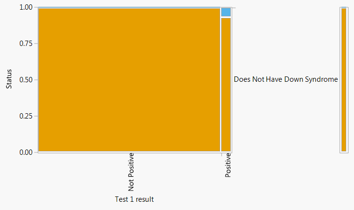 7.8. The plot on the left represents conditioning on Down Syndrome status, while the plot on the right represents conditioning on test result." width="40%" />
Recall Bayes rule for multiple cases. \[\begin{align*} \textrm{P}(C_j|A) & = \frac{\textrm{P}(A|C_j)\textrm{P}(C_j)}{\sum_{j=1}^k \textrm{P}(A|C_i) \textrm{P}(C_i)}\\ & = \frac{\textrm{P}(A|C_j)\textrm{P}(C_j)}{\textrm{P}(A)}\\ & \propto \textrm{P}(A|C_j)\textrm{P}(C_j) \end{align*}\]
Recall that \(C_j\) represents a “hypothesis” and \(A\) represents “evidence”. The probability \(\textrm{P}(A |C_j)\) is called the likelihood127 of observing evidence \(A\) given hypothesis \(C_j\).
The marginal probability of the evidence, \(\textrm{P}(A)\), in the denominator (which can be calculated using the law of total probability) simply normalizes the numerators to ensure that the updated probabilities \(\textrm{P}(C_j|A)\) sum to 1 when summing over all the cases. Thus Bayes rule says that the posterior probability \(\textrm{P}(C_j|A)\) is proportional to the product of the likelihood \(\textrm{P}(A | B_j)\) and the prior probability \(\textrm{P}(C_j)\). \[\begin{align*} \textrm{P}(C_j | A) & \propto \textrm{P}(A|C_j)\textrm{P}(C_j)\\ \text{posterior} & \propto \text{likelihood} \times \text{prior} \end{align*}\]
As an illustration, consider Example 7.4. Suppose we are given that the randomly selected person supports impeachment, and we want to update our probabilities for the person’s party affiliation. The following organizes the calculations in a Bayes’ table which illustrates “posterior is proportional to likelihood times prior”.
| Prior | Likelihood (of supporting impeachment) | Prior \(\times\) Likelihood | Posterior | |
|---|---|---|---|---|
| Democrat | 0.31 | 0.83 | (0.31)(0.83) = 0.2573 | \(\frac{0.2573}{0.4739} = 0.543\) |
| Independent | 0.40 | 0.44 | (0.40)(0.44) = 0.1760 | \(\frac{0.1760}{0.4739} = 0.371\) |
| Republican | 0.29 | 0.14 | (0.29)(0.14) = 0.0406 | \(\frac{0.4060}{0.4739} = 0.086\) |
| Sum | 1.00 | NA | 0.4739 | 1.000 |
The product of prior and likelihood for Democrats (0.2573) is 6.34 (0.2573/0.0406) times higher than the product of prior and likelihood for Republicans (0.0406). Therefore, Bayes rule implies that the conditional probability that the person is a Democrat given support for impeachment should be 6.34 times higher than the conditional probability that the person is a Republican given support for impeachment. Similarly, the conditional probability that the person is a Democrat given support for impeachment should be 1.46 (0.2573/0.1760) times higher than the conditional probability that the person is an Independent given support for impeachment, and the conditional probability that the person is an Independent given support for impeachment should be 4.33 (0.1760/0.0406) times higher than the conditional probability that the person is a Republican given support for impeachment. The last column just translates these relative relationships into probabilities that sum to 1.
You should really click on this birthday problem link.↩︎
Which isn’t quite true. However, a non-uniform distribution of birthdays only increases the probability that at least two people have the same birthday. To see that, think of an extreme case like if everyone were born in September.↩︎
Source: http://www.cdc.gov/ncbddd/birthdefects/downsyndrome/data.html↩︎
Estimates of these probabilities vary between different sources. The values in the exercise were based on https://www.ncbi.nlm.nih.gov/pubmed/17350315↩︎
“Likelihood” here is used in the statistical sense, as in “maximum likelihood estimation”, rather than as a loose synonymn for the word probability.↩︎