15.1 Statistical Analysis of Portfolios: Two Assets
Most of the issues involved with the statistical analysis of portfolios can be illustrated in the simple case of a two asset portfolio. Let \(R_{A}\) and \(R_{B}\) denote the simple returns on two risky assets and assume these returns are characterized by the CER model: \[\begin{equation} \left(\begin{array}{c} R_{A}\\ R_{B} \end{array}\right)\sim N\left(\left(\begin{array}{c} \mu_{A}\\ \mu_{B} \end{array}\right),\,\left(\begin{array}{cc} \sigma_{A}^{2} & \sigma_{AB}\\ \sigma_{AB} & \sigma_{B}^{2} \end{array}\right)\right)\tag{15.1} \end{equation}\] In matrix notation we have: \[ \mathbf{R}\sim N(\mu,\,\Sigma), \] where \[ \mathbf{R}=\left(\begin{array}{c} R_{A}\\ R_{B} \end{array}\right),\,\mu=\left(\begin{array}{c} \mu_{A}\\ \mu_{B} \end{array}\right),\,\Sigma=\left(\begin{array}{cc} \sigma_{A}^{2} & \sigma_{AB}\\ \sigma_{AB} & \sigma_{B}^{2} \end{array}\right) \] A portfolio with weight vector \(\mathbf{x}=(x_{A},x_{B})^{\prime}\) has return \(R_{p}=\mathbf{x}^{\prime}\mathbf{R}=x_{A}R_{A}+x_{B}R_{B}\) which is also described by the CER model \[\begin{eqnarray*} R_{p} & \sim & N(\mu_{p},\,\sigma_{p}^{2}),\\ \mu_{p} & = & \mathbf{x}^{\prime}\mu=x_{A}\mu_{A}+x_{B}\mu_{B},\\ \sigma_{p}^{2} & = & \mathbf{x}^{\prime}\mathbf{\varSigma}\mathbf{x}=x_{A}^{2}\sigma_{A}^{2}+x_{B}^{2}\sigma_{B}^{2}+2x_{A}x_{B}\sigma_{AB}. \end{eqnarray*}\] We observe a sample of asset returns of size \(T\), \(\{r_{t}\}_{t=1}^{T}\), where \(\mathbf{r}_{t}=(r_{At},r_{Bt})^{\prime}\), that we assume is generated from the CER model (15.1) from which we create the sample portfolio returns \(r_{p,t}=\mathbf{x}^{\prime}\mathbf{r}_{t}=x_{A}r_{At}+x_{B}r_{Bt}\).
The true CER model parameters are unknown in practice and must be estimated from the observed data. From chapter xxx, the CER model parameter estimates are the corresponding sample statistics: \[\begin{align} & \hat{\mu}_{i}=\frac{1}{T}\sum_{t=1}^{T}r_{it},\,\hat{\sigma}_{i}^{2}=\frac{1}{T-1}\sum_{t=1}^{T}(r_{it}-\hat{\mu}_{i})^{2}, \nonumber \\ & \hat{\sigma}_{i}=\sqrt{\hat{\sigma}_{i}^{2}},\,\hat{\sigma}_{ij}^{2}=\frac{1}{T-1}\sum_{t=1}^{T}(r_{it}-\hat{\mu}_{i})(r_{jt}-\hat{\mu}_{j}).\tag{15.2} \end{align}\] These estimates are unbiased, asymptotically normally distributed, and have estimation errors which can be quantified by standard errors and 95% confidence intervals.94 For \(\hat{\mu}_{i}\), \(\hat{\sigma}_{i}^{2}\), \(\hat{\sigma}_{i}\) we have analytic standard error formulas: \[\begin{equation} \mathrm{se}(\hat{\mu}_{i})=\frac{\sigma_{i}}{\sqrt{T}},\,\mathrm{se}(\hat{\sigma}_{i}^{2})\approx\frac{\sigma_{i}^{2}}{\sqrt{T/2}},\,\mathrm{se}(\hat{\sigma}_{i})\approx\frac{\sigma_{i}}{\sqrt{2T}}.\tag{15.3} \end{equation}\] For \(\hat{\sigma}_{ij}^{2}\) there is no easy formula but we can use the bootstrap to compute a numerical estimate of the standard error. For 95% confidence intervals, we use the rule of thumb “estimate \(\pm\) 2\(\times\)standard error” .
We can estimate the CER model parameters \(\mu_{p}\), \(\sigma_{p}^{2}\) and \(\sigma_{p}\) for the portfolio return, \(R_{p}\), using two equivalent methods. In the first method, we use the sample portfolio returns \(\{r_{p,t}\}_{t=1}^{T}\) and compute sample statistics: \[\begin{equation} \hat{\mu}_{p}=\frac{1}{T}\sum_{t=1}^{T}r_{p,t},\,\hat{\sigma}_{p}^{2}=\frac{1}{T-1}\sum_{t=1}^{T}(r_{p,t}-\hat{\mu}_{p})^{2},\,\hat{\sigma}_{p}=\sqrt{\hat{\sigma}_{p}^{2}}.\tag{15.4} \end{equation}\] These estimates are unbiased and asymptotically normal with standard errors: \[\begin{equation} \mathrm{se}(\hat{\mu}_{p})=\frac{\sigma_{p}}{\sqrt{T}},\,\mathrm{se}(\hat{\sigma}_{p}^{2})\approx\frac{\sigma_{p}^{2}}{\sqrt{T/2}},\,\mathrm{se}(\hat{\sigma}_{p})\approx\frac{\sigma_{p}}{\sqrt{2T}}.\tag{15.5} \end{equation}\] In the second method, we compute estimates of \(\mu_{p}\) and \(\sigma_{p}^{2}\) directly from the individual asset estimates in (15.2): \[\begin{eqnarray} \hat{\mu}_{p} & = & \mathbf{x}^{\prime}\hat{\mu}=x_{A}\hat{\mu}_{A}+x_{B}\hat{\mu}_{B},\tag{15.6}\\ \hat{\sigma}_{p}^{2} & = & x^{\prime}\widehat{\Sigma}x=x_{A}^{2}\hat{\sigma}_{A}^{2}+x_{B}^{2}\hat{\sigma}_{B}^{2}+2x_{A}x_{B}\hat{\sigma}_{AB}.\tag{15.7} \end{eqnarray}\] The estimates of \(\mu_{p}\) and \(\sigma_{p}^{2}\) in (15.6) and (15.7), respectively, are numerically identical to the estimates in (15.4). To see this, consider the calculation of \(\hat{\mu}_{p}\) in (15.6): \[\begin{eqnarray*} \hat{\mu}_{p} & = & x_{A}\hat{\mu}_{A}+x_{B}\hat{\mu}_{B}=x_{A}\left(\frac{1}{T}\sum_{t=1}^{T}r_{At}\right)+x_{B}\left(\frac{1}{T}\sum_{t=1}^{T}r_{Bt}\right)\\ & = & \frac{1}{T}\sum_{t=1}^{T}(x_{A}r_{At}+x_{B}r_{Bt})=\frac{1}{T}\sum_{t=1}^{T}r_{p,t}. \end{eqnarray*}\] The proof of the equivalence of \(\hat{\sigma}_{p}^{2}\) in (15.7) with \(\hat{\sigma}_{p}^{2}\) in (15.4) is left as an end-of-chapter exercise.
The standard errors of \(\hat{\mu}_{p}\) and \(\hat{\sigma}_{p}^{2}\) can also be directly calculated from (15.6) and (15.7). Consider the calculation for \(\mathrm{se}(\hat{\mu}_{p})\): \[\begin{equation} \mathrm{var}(\hat{\mu}_{p})=\mathrm{var}(x_{A}\hat{\mu}_{A}+x_{B}\hat{\mu}_{B})=x_{A}^{2}\mathrm{var}(\hat{\mu}_{A})+x_{B}^{2}\mathrm{var}(\hat{\mu}_{B})+2x_{A}x_{B}\mathrm{cov}(\hat{\mu}_{A},\hat{\mu}_{B}).\tag{15.8} \end{equation}\] Now, from chapter ??, \[ \mathrm{var}(\hat{\mu}_{A})=\frac{\sigma_{A}^{2}}{T},\,\mathrm{var}(\hat{\mu}_{B})=\frac{\sigma_{B}^{2}}{T}. \] However, what is \(\mathrm{cov}(\hat{\mu}_{A},\hat{\mu}_{B})\)? It can be shown that \[ \mathrm{cov}(\hat{\mu}_{A},\hat{\mu}_{B})=\frac{\sigma_{AB}}{T}. \] Then (15.8) can be rewritten as \[\begin{eqnarray*} \mathrm{var}(\hat{\mu}_{p}) & = & x_{A}\frac{\sigma_{A}^{2}}{T}+x_{B}\frac{\sigma_{B}^{2}}{T}+2x_{A}x_{B}\frac{\sigma_{AB}}{T}\\ & = & \frac{1}{T}\left(x_{A}^{2}\sigma_{A}^{2}+x_{B}^{2}\sigma_{B}^{2}+2x_{A}x_{B}\sigma_{AB}\right)\\ & = & \frac{\sigma_{p}^{2}}{T} \end{eqnarray*}\] Hence, \[ \mathrm{se}(\hat{\mu}_{p})=\sqrt{\mathrm{var}(\hat{\mu}_{p})}=\frac{\sigma_{p}}{\sqrt{T}} \] which is the same formula given in (15.5).
Unfortunately, the calculation of \(\mathrm{se}(\hat{\sigma}_{p}^{2})\) is a bit horrific and we only sketch out some of the details. Now, \[\begin{eqnarray} \mathrm{var}(\hat{\sigma}_{p}^{2}) & = & \mathrm{var}(x_{A}^{2}\hat{\sigma}_{A}^{2}+x_{B}^{2}\hat{\sigma}_{B}^{2}+2x_{A}x_{B}\hat{\sigma}_{AB})\tag{15.9}\\ & = & x_{A}^{4}\mathrm{var}(\hat{\sigma}_{A}^{2})+x_{B}^{4}\mathrm{var}(\hat{\sigma}_{B}^{2})+4x_{A}^{2}x_{B}^{2}\mathrm{var}(\hat{\sigma}_{AB})\nonumber \\ & & +2x_{A}^{2}x_{B}^{2}\mathrm{cov}(\hat{\sigma}_{A}^{2},\hat{\sigma}_{B}^{2})+4x_{A}^{3}x_{B}\mathrm{cov}(\hat{\sigma}_{A}^{2},\hat{\sigma}_{AB})\nonumber \\ & & +4x_{A}x_{B}^{3}\mathrm{cov}(\hat{\sigma}_{B}^{2},\hat{\sigma}_{AB})\nonumber \end{eqnarray}\] Unfortunately, there are no easy formulas for \(\mathrm{var}(\hat{\sigma}_{AB})\), \(\mathrm{cov}(\hat{\sigma}_{A}^{2},\hat{\sigma}_{B}^{2})\), \(\mathrm{cov}(\hat{\sigma}_{A}^{2},\hat{\sigma}_{AB})\) and \(\mathrm{cov}(\hat{\sigma}_{B}^{2},\hat{\sigma}_{AB})\). With a CLT approximation and much tedious calculation it can be shown that (15.9) is approximately equal to the square of \(\mathrm{se}(\hat{\sigma}_{p}^{2})\) given in (15.5). Obviously, the method of computing standard errors for \(\hat{\mu}_{p}\) and \(\hat{\sigma}_{p}^{2}\) directly from the CER model estimates computed from the sample portfolio returns is much easier than the indirect calculations based on the individual asset estimates.
To be completed… table example data
Table 11.1 gives annual return distribution parameters for two hypothetical assets \(A\) and \(B\). We use this distribution but re-scale the values to represent a monthly return distribution. Asset \(A\) is the high risk asset with a monthly return of \(\mu_{A}=1.46\%\) and monthly standard deviation of \(\sigma_{A}=7.45\%\). Asset B is a lower risk asset with monthly return \(\mu_{B}=0.458\%\) and monthly standard deviation of \(\sigma_{B}=3.32\%\). The assets are assumed to be slightly negatively correlated with correlation coefficient \(\rho_{AB}=-0.164\). Given the standard deviations and the correlation, the covariance can be determined from \(\sigma_{AB}=\rho_{AB}\sigma_{A}\sigma_{B}=-0.0004\). In R, these CER model parameters are created using:
mu.A = 0.175/12
sig.A = 0.258/sqrt(12)
sig2.A = sig.A^2
mu.B = 0.055/12
sig.B = 0.115/sqrt(12)
sig2.B = sig.B^2
rho.AB = -0.164
sig.AB = rho.AB*sig.A*sig.B
sigma.mat = matrix(c(sig2.A, sig.AB, sig.AB, sig2.B),
                   2, 2, byrow=TRUE)
mu.vec = c(mu.A, mu.B)
sd.vec = c(sig.A, sig.B)
names(mu.vec) = names(sd.vec) = c("asset.A", "asset.B")
dimnames(sigma.mat) = list(names(mu.vec), names(mu.vec))
For portfolio analysis, we consider an equally weighted portfolio of assets A and B. The CER model parameters for this portfolio are:
x1.A = 0.5
x1.B = 1 - x1.A
x1.vec = c(x1.A, x1.B)
names(x1.vec) = names(mu.vec)
mu.p1 = x1.A*mu.A + x1.B*mu.B
sig2.p1 = x1.A^2 * sig2.A + x1.B^2 * sig2.B + 2*x1.A*x1.B*sig.AB
sig.p1 = sqrt(sig2.p1)
cbind(mu.p1, sig2.p1, sig.p1)
## mu.p1 sig2.p1 sig.p1
## [1,] 0.009583333 0.001459526 0.03820374We use the above CER model parameters to simulate \(T=60\) hypothetical returns for assets A and B and the equally weighted portfolio:
library(mvtnorm)
n.obs = 60
set.seed(125)
returns.sim = rmvnorm(n.obs, mean=mu.vec, sigma=sigma.mat)
colnames(returns.sim) = names(mu.vec)
rp1.sim = returns.sim%*%x1.vec
The estimates of the CER model parameters from the simulated returns for the individual assets are:
muhat.vals = colMeans(returns.sim)
sig2hat.vals = apply(returns.sim, 2, var)
sigmahat.vals = apply(returns.sim, 2, sd)
covmat.hat = cov(returns.sim)
covhat = covmat.hat[1,2]
rbind(muhat.vals, sig2hat.vals, sigmahat.vals)
## asset.A asset.B
## muhat.vals 0.030771398 0.002117967
## sig2hat.vals 0.005393922 0.001267304
## sigmahat.vals 0.073443325 0.035599210## [1] -0.0008477922The estimated standard errors and 95% confidence intervals for \(\hat{\mu}_{i}\) and \(\hat{\sigma}_{i}\) \((i=A,\,B)\) are:
# estimated standard errors
se.muhat = sigmahat.vals/sqrt(n.obs)
se.sigmahat = sigmahat.vals/sqrt(2*n.obs)
rbind(se.muhat, se.sigmahat)
## asset.A asset.B
## se.muhat 0.009481492 0.004595838
## se.sigmahat 0.006704428 0.003249748# 95% confidence intervals
lower.mu = muhat.vals - 2*se.muhat
upper.mu = muhat.vals + 2*se.muhat
lower.sigma = sigmahat.vals - 2*se.sigmahat
upper.sigma = sigmahat.vals + 2*se.sigmahat
cbind(lower.mu, upper.mu) ## lower.mu upper.mu
## asset.A 0.01180841 0.04973438
## asset.B -0.00707371 0.01130964## lower.sigma upper.sigma
## asset.A 0.06003447 0.08685218
## asset.B 0.02909971 0.04209871Here, we see that the means are not estimated as precisely as the volatilities and that all of the true values are contained in the 95% confidence intervals.
For the equally weighted portfolio, the CER model estimates computed directly from the simulated portfolio returns using (15.4) are:
muhat.p1 = mean(rp1.sim)
sig2hat.p1 = as.numeric(var(rp1.sim))
sigmahat.p1 = sd(rp1.sim)
cbind(muhat.p1, sig2hat.p1, sigmahat.p1)
## muhat.p1 sig2hat.p1 sigmahat.p1
## [1,] 0.01644468 0.00124141 0.03523365The portfolio estimates computed from the asset estimates (15.6) and (15.7) are numerically equivalent:
muhat.p1 = as.numeric(x1.A*muhat.vals[1] + x1.B*muhat.vals[2])
sig2hat.p1 = as.numeric(x1.A^2 * sig2hat.vals[1] +
                        x1.B^2 * sig2hat.vals[2] +
                        2*x1.A*x1.B*covhat)
sighat.p1 = sqrt(sig2hat.p1)
cbind(muhat.p1, sig2hat.p1, sigmahat.p1)
## muhat.p1 sig2hat.p1 sigmahat.p1
## [1,] 0.01644468 0.00124141 0.03523365The estimated standard errors for \(\hat{\mu}_{p}\) and \(\hat{\sigma}_{p}\), and 95% confidence intervals for \(\mu_{p}\) and \(\sigma_{p}\) computed using (15.5) are:
# estimated standard errors
se.muhat.p1 = sigmahat.p1/sqrt(n.obs)
se.sigmahat.p1 = sigmahat.p1/sqrt(2*n.obs)
cbind(se.muhat.p1, se.sigmahat.p1)
## se.muhat.p1 se.sigmahat.p1
## [1,] 0.004548645 0.003216378# 95% confidence intervals
lower.mu = muhat.p1 - 2*se.muhat.p1
upper.mu = muhat.p1 + 2*se.muhat.p1
lower.sigma = sigmahat.p1 - 2*se.sigmahat.p1
upper.sigma = sigmahat.p1 + 2*se.sigmahat.p1
ans = rbind(c(lower.mu, upper.mu),
c(lower.sigma, upper.sigma))
colnames(ans) = c("lower", "upper")
rownames(ans) = c("mu.p", "sigma.p")
ans## lower upper
## mu.p 0.007347392 0.02554197
## sigma.p 0.028800898 0.04166641As with the individual assets, the portfolio mean is estimated less precisely than the portfolio volatility and the true values are in the 95% confidence intervals.
\(\blacksquare\)
In our analysis of portfolios, we visualized the risk return trade-off between portfolios by plotting the volatility-expected return pairs \((\hat{\sigma}_{p},\,\hat{\mu}_{p})\) of different portfolios. We did this without considering estimation error in \(\hat{\sigma}_{p}\) and \(\hat{\mu}_{p}\). Estimation error in\(\hat{\sigma}_{p}\) and \(\hat{\mu}_{p}\) creates uncertainty about the location of the true values \((\sigma_{p},\,\mu_{p})\) in the risk-return diagram.
Figure 15.1 shows the true values and sample estimates of the pairs \((\sigma_{A},\mu_{A}),\) \((\sigma_{B},\mu_{B})\), and \((\sigma_{p},\mu_{p})\) for the equally weighted portfolio created using:
# true values
plot(sd.vec, mu.vec, pch=16, col="black",
     ylim=c(-0.01, 0.04), xlim=c(0, 0.1),
     xlab=expression(sigma[p]), ylab=expression(mu[p]),
     cex=2)
abline(h=0)
points(sig.p1, mu.p1, pch=16, col="black", cex=2)
text(x=sig.A, y=mu.A, labels="A", pos=4, cex = 1.5)
text(x=sig.B, y=mu.B, labels="B", pos=4, cex = 1.5)
text(x=sig.p1, y=mu.p1, labels="P", pos=4, cex = 1.5)
# estimates
points(sigmahat.vals, muhat.vals, pch=16, col="blue", cex=2)
points(sigmahat.p1, muhat.p1, pch=16, col="blue", cex=2)
text(x=sigmahat.vals[1], y=muhat.vals[1], labels="A Hat",
     col="blue", pos=4, cex = 1.5)
text(x=sigmahat.vals[2], y=muhat.vals[2], labels="B Hat",
     col="blue", pos=4, cex = 1.5)
text(x=sigmahat.p1, y=muhat.p1, labels="P Hat",
     col="blue", pos=4, cex = 1.5)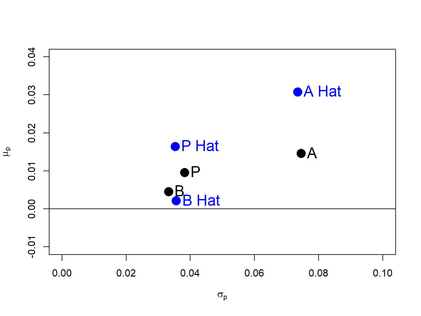
Figure 15.1: Risk-return diagram for example data. \(\mathrm{A}=(\sigma_{A},\mu_{A})\), \(\mathrm{B}=(\sigma_{B},\mu_{B})\), \(\mathrm{A~Hat}=(\hat{\sigma}_{A},~\hat{\mu}_{A})\), \(\mathrm{B~Hat}=(\hat{\sigma}_{B},~\hat{\mu}_{B})\).
We see that \((\hat{\sigma}_{B},\hat{\mu}_{B})\) is fairly close to \((\sigma_{B},\mu_{B})\) but that \((\hat{\sigma}_{A},\hat{\mu}_{A})\) is quite far above \((\sigma_{A},\mu_{A})\) and \((\hat{\sigma}_{P},\hat{\mu}_{P})\) is moderately far above \((\sigma_{P},\mu_{P})\). The large positive estimation errors in \(\hat{\mu}_{P}\) and \(\hat{\mu}_{A}\) greatly overstate the risk-return characteristics of the equally weighted portfolio and asset A.
\(\blacksquare\)
To illustrate estimation error in the risk return diagram, the individual 95% confidence intervals for \(\mu_{i}\) and \(\sigma_{i}\) could be superimposed on the plot as rectangles centered at the pairs \((\hat{\sigma}_{i},\hat{\mu}_{i})\). However, the probability that these rectangles contain the true pairs \((\sigma_{i},\mu_{i})\) is not equal to 95% because the confidence intervals for \(\mu_{i}\) are created independently from the confidence intervals for \(\sigma_{i}\). To create a joint confidence set that cover the pair \((\sigma_{i},\mu_{i})\) with probability 95% requires knowing the joint probability distribution of \((\hat{\sigma}_{i},\hat{\mu}_{i})\). In chapter ??, it was shown that in the CER model: \[\begin{equation} \left(\begin{array}{c} \hat{\sigma}_{i}\\ \hat{\mu}_{i} \end{array}\right)\sim N\left(\left(\begin{array}{c} \sigma_{i}\\ \mu_{i} \end{array}\right),\left(\begin{array}{cc} \mathrm{se}(\hat{\sigma}_{i})^{2} & 0\\ 0 & \mathrm{se}(\hat{\mu}_{i})^{2} \end{array}\right)\right)\tag{15.10} \end{equation}\] for large enough \(T\). Hence, \(\hat{\sigma}_{i}\) and \(\hat{\mu}_{i}\) are (asymptotically) jointly normally distributed and \(\mathrm{cov}(\hat{\sigma}_{i},\hat{\mu}_{i})=0\) which implies that they are also independent. Let \(\theta=(\sigma_{i},\mu_{i})^{\prime},\,\)\(\hat{\theta}=(\hat{\sigma}_{i},\hat{\mu}_{i})^{\prime}\) and \(\mathbf{V}=\mathrm{diag}(\mathrm{se}(\hat{\sigma}_{i})^{2},\mathrm{se}(\hat{\mu}_{i})^{2})\). Then (15.10) can be expressed as \(\hat{\theta}\sim N(\theta,\,\mathbf{V})\). It follows that the quadratic form \(\left(\hat{\theta}-\theta\right)^{\prime}\mathbf{V}^{-1}\left(\hat{\theta}-\theta\right)\sim\chi^{2}(2),\) and so \[\begin{equation} Pr\left\{ \left(\hat{\theta}-\theta\right)^{\prime}\mathbf{V}^{-1}\left(\hat{\theta}-\theta\right)\leq q_{.95}^{\chi^{2}(2)}\right\} =0.95\tag{15.11} \end{equation}\] where \(q_{.95}^{\chi^{2}(2)}\) is the 95% quantile of the \(\chi^{2}(2)\) distribution. The equation \(\left(\hat{\theta}-\theta\right)^{\prime}\mathbf{V}^{-1}\left(\hat{\theta}-\theta\right)=q_{.95}^{\chi^{2}(2)}\) defines an un-tilted ellipse in \(\sigma_{i}-\mu_{i}\) space centered at \((\hat{\sigma}_{i},\hat{\mu}_{i})\) with axes proportional to \(\mathrm{se}(\hat{\sigma}_{i})\) and \(\mathrm{se}(\hat{\mu}_{i})\), respectively. This ellipse is the joint 95% confidence set for \((\sigma_{i},\mu_{i})\).
Figure 15.2 repeats Figure 15.1 with the addition of the joint confidence sets for \((\sigma_{A},\mu_{A}),\) \((\sigma_{B},\mu_{B})\), and \((\sigma_{p},\mu_{p})\) , created using
##
## Attaching package: 'ellipse'
## The following object is masked from 'package:graphics':
##
## pairsplot(sd.vec, mu.vec, pch=16, col="black",
ylim=c(-0.01, 0.06), xlim=c(0, 0.1),
xlab=expression(sigma[p]), ylab=expression(mu[p]),cex=2)
abline(h=0)
points(sig.p1, mu.p1, pch=16, col="black", cex=2)
text(x=sig.A, y=mu.A, labels="A", pos=4, cex = 1.5)
text(x=sig.B, y=mu.B, labels="B", pos=4, cex = 1.5)
text(x=sig.p1, y=mu.p1, labels="P", pos=4, cex = 1.5)
# estimates points(sigmahat.vals, muhat.vals,
# pch=16, col="blue", cex=2)
points(sigmahat.p1, muhat.p1, pch=16, col="blue", cex=2)
text(x=sigmahat.vals[1], y=muhat.vals[1], labels="A Hat",
col="blue", pos=4, cex = 1.5)
text(x=sigmahat.vals[2], y=muhat.vals[2], labels="B Hat",
col="blue", pos=4, cex = 1.5)
text(x=sigmahat.p1, y=muhat.p1, labels="P Hat",
col="blue", pos=4, cex = 1.5)
# Create asymptotic variances
V.A = matrix(c(se.sigmahat[1]^2, 0 ,0,
se.muhat[1]^2), 2, 2, byrow=TRUE)
V.B = matrix(c(se.sigmahat[2]^2, 0 ,0,
se.muhat[2]^2), 2, 2, byrow=TRUE)
V.P = matrix(c(se.sigmahat.p1^2, 0 ,0,
se.muhat.p1^2), 2, 2, byrow=TRUE)
# plot confidence ellipses
lines(ellipse(V.A, centre=c(sigmahat.vals[1],
muhat.vals[1]), level=0.95),
col="red" , lwd=2)
lines(ellipse(V.B, centre=c(sigmahat.vals[2],
muhat.vals[2]), level=0.95),
col="red", lwd=2 )
lines(ellipse(V.P, centre=c(sigmahat.p1,
muhat.p1), level=0.95),
col="red", lwd=2 )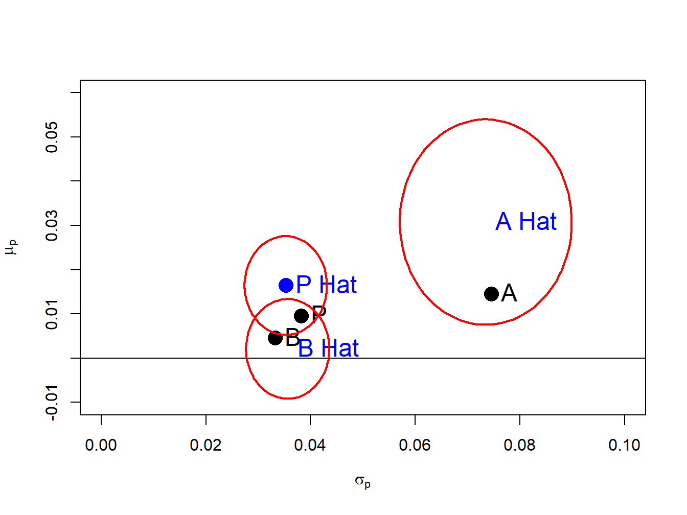
Figure 15.2: Risk return tradeoff with 95% confidence ellipses
The ellipse() function from the R package ellipse
is used to draw the 95% confidence sets. The confidence ellipses
are longer in the \(\mu_{i}\) direction because \(\mathrm{se}(\hat{\mu}_{i})\)
is larger than \(\mathrm{se}(\hat{\sigma}_{i})\) and indicate more
uncertainty about the true values of \(\mu_{i}\) than the true values
of \(\sigma_{i}.\) The ellipse for \((\sigma_{A},\mu_{A})\) is much
bigger than the ellipses for \((\sigma_{B},\mu_{B})\) and \((\sigma_{p},\mu_{p})\)
and indicates a wide range of possible values for \((\sigma_{A},\mu_{A})\)
. For all pairs, the true values are inside the 95% confidence ellipses.95
\(\blacksquare\)
The estimation errors in the points \((\hat{\sigma}_{i},\hat{\mu}{}_{i})\) can also be illustrated using the bootstrap. We simply sample with replacement from the observed returns \(B\) times and compute estimates of \((\sigma_{i},\mu_{i})\) from each bootstrap sample. We can then plot the \(B\) bootstrap pairs \((\hat{\sigma}_{i}^{*},\hat{\mu}_{i}^{*})\) on the risk return diagram instead of the confidence ellipses.
The following R code creates \(B=500\) bootstrap estimates of \((\sigma_{i},\mu_{i})\) for \(i=A,B,P\):
n.boot = 500
mu.boot = matrix(0, n.boot, 3)
sd.boot = matrix(0, n.boot, 3)
colnames(mu.boot) = colnames(sd.boot) = c("A", "B", "P")
set.seed(123)
for (i in 1:n.boot) {
   boot.idx = sample(n.obs, replace=TRUE)
   ret.boot = returns.sim[boot.idx, ]
   rp1.boot = ret.boot%*%x1.vec
   ret.boot = cbind(ret.boot, rp1.boot)
   mu.boot[i, ] = colMeans(ret.boot)
   sd.boot[i, ] = apply(ret.boot, 2, sd)
}
Figure 15.3 repeats Figure 15.2 and adds the bootstrap estimates of \((\sigma_{i},\mu_{i})\) for \(i=A,B,P\). Notice that the bootstrap estimates for each asset produce a scatter that fills the 95% confidence ellipses with just a few estimates lying outside the ellipses. Hence, the bootstrap is an easy and effective way to illustrate estimation error in the risk-return diagram.
\(\blacksquare\)
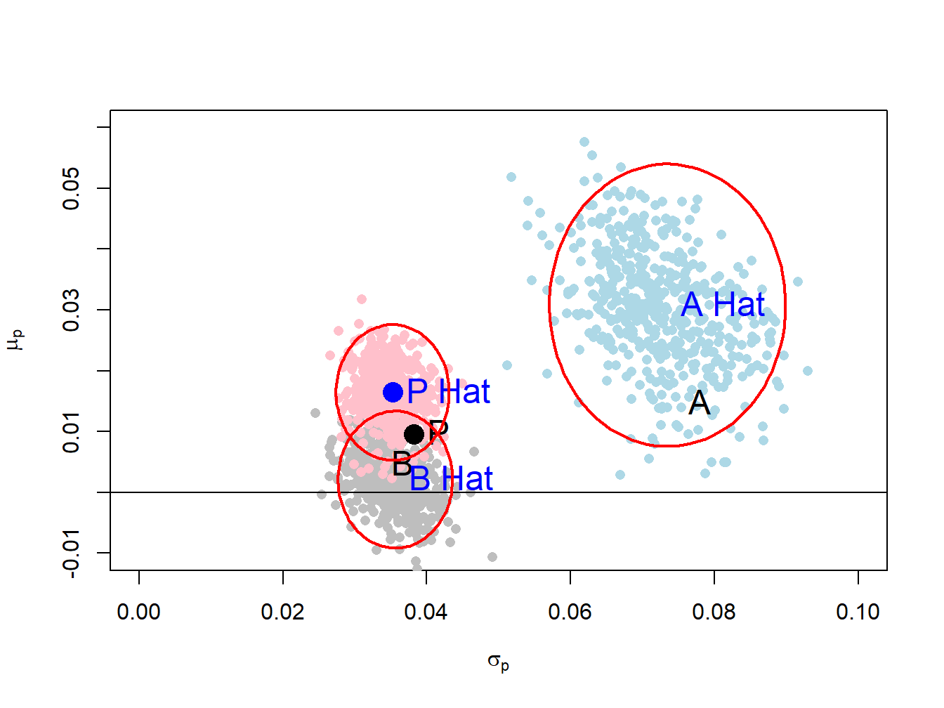
Figure 15.3: Risk return trade off with bootstrap estimates.
15.1.1 Estimation error in the portfolio frontier
In the case of two risky assets, the portfolio frontier is a plot of the risk-return characteristics of all feasible portfolios. From this frontier, we can readily determine the set of efficient portfolios which are those portfolios that have the highest expected return for a given risk level. If we construct the portfolio frontier from portfolio risk and return estimates from the CER model, then the estimation error in these estimates leads to estimation error in the entire portfolio frontier.
Using the example data, we can construct the true unobservable portfolio frontier as well as an estimate of this frontier from the simulated returns. For example, consider creating the true and estimated portfolio frontiers for the following portfolios:
The risk-return characteristics of the portfolios on the true portfolio frontier are:
mu.p = x.A*mu.A + x.B*mu.B
sig2.p = x.A^2 * sig2.A + x.B^2 * sig2.B + 2*x.A*x.B*sig.AB
sig.p = sqrt(sig2.p)
The risk-return characteristics of the portfolios on the estimated frontier are:
muhat.p = x.A*muhat.vals["asset.A"] + x.B*muhat.vals["asset.B"]
sig2hat.p = x.A^2 * sig2hat.vals["asset.A"] +
   x.B^2 * sig2hat.vals["asset.B"] + 2*x.A*x.B*covhat
sighat.p = sqrt(sig2hat.p)
The true and estimated portfolios are illustrated in Figure 15.4, created with
plot(sig.p, mu.p, pch=16, type="b", col="black",
     ylim=c(-0.01, 0.041), xlim=c(0, 0.125),
     xlab=expression(sigma[p]), ylab=expression(mu[p]), cex=1)
abline(h=0)
points(sd.vec, mu.vec, pch=16, col="black", cex=2)
text(x=sig.A, y=mu.A, labels="A", pos=3, cex = 1.5)
text(x=sig.B, y=mu.B, labels="B", pos=3, cex = 1.5)
# estimated assets and frontier
points(sighat.p, muhat.p, type="b", pch=16, col="blue", cex=1)
points(sigmahat.vals, muhat.vals, pch=16, col="blue", cex=2)
text(x=sigmahat.vals[1], y=muhat.vals[1], labels="A Hat",
     col="blue", pos=3, cex = 1.5)
text(x=sigmahat.vals[2], y=muhat.vals[2], labels="B Hat",
     col="blue", pos=2, cex = 1.5)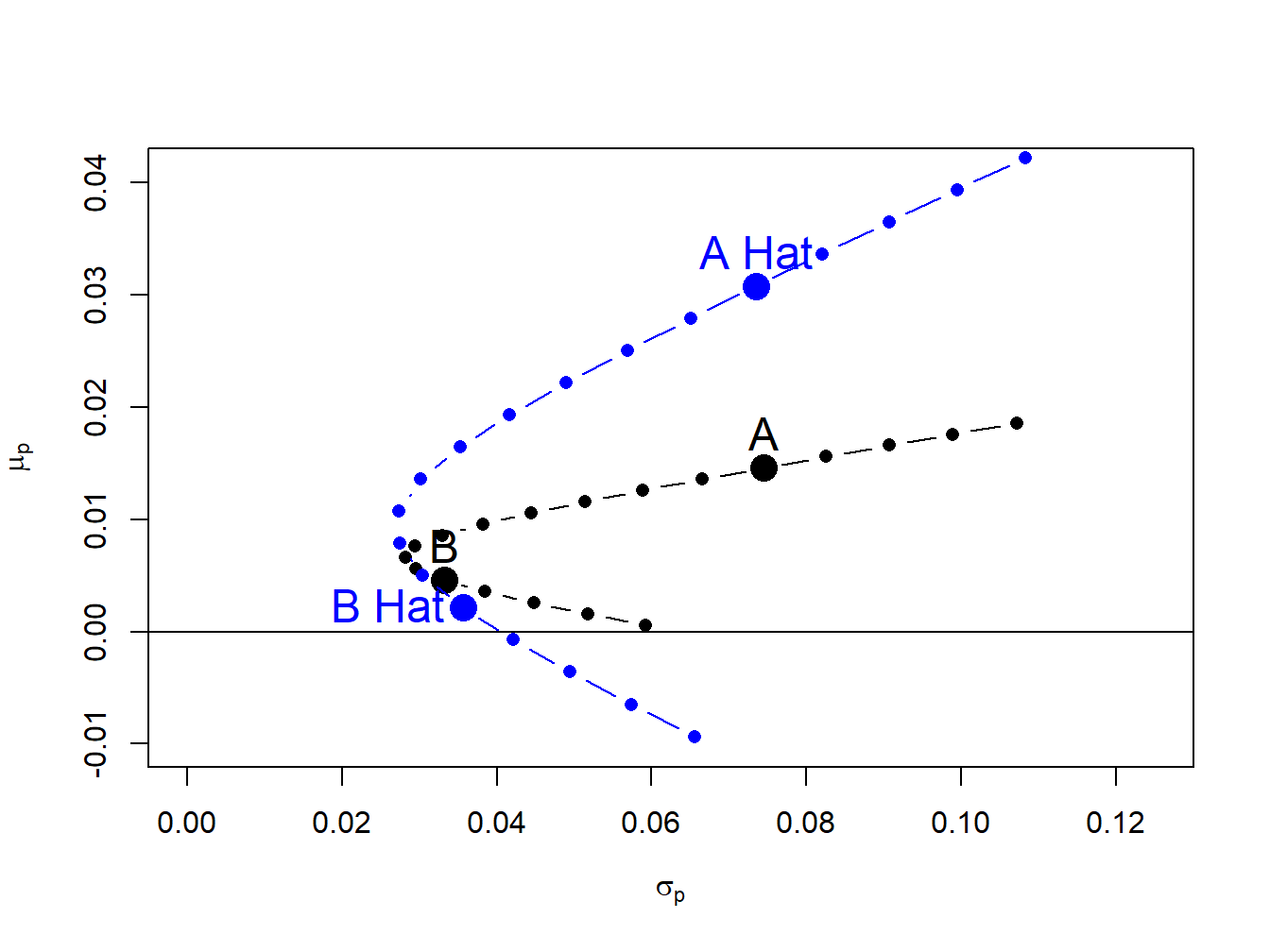
Figure 15.4: True and estimated portfolio frontiers
Due to the large estimation error in \(\hat{\mu}_{A}\), the estimated frontier is considerably higher than the true frontier. As a result, portfolios on the estimated frontier appear to have higher reward-to-risk properties than they actually do.
\(\blacksquare\)
Sampling uncertainty about the estimated frontier can be easily computed using the bootstrap. The process is the same as in the case of a single asset. For each bootstrap sample, estimate the expected return and volatility of each portfolio on the frontier and then plot these bootstrap pairs on the plot showing the estimated frontier from the sample returns.
The R code to create \(B=1000\) bootstrap estimates of risk and return pairs for the frontier portfolios is
# initialize matrices
n.boot = 1000
mu.boot = matrix(0, n.boot, length(x.A))
sd.boot = matrix(0, n.boot, length(x.A))
colnames(mu.boot) = colnames(sd.boot) =
      paste("P", 1:length(x.A), sep=".")
# bootstrap loop
set.seed(123)
for (i in 1:n.boot) {
   boot.idx = sample(n.obs, replace=TRUE)
   ret.boot = returns.sim[boot.idx, ]
# CER model estimates
   muhat.boot = colMeans(ret.boot)
   sig2hat.boot = apply(ret.boot, 2, var)
   sigmahat.boot = sqrt(sig2hat.boot)
   covhat.boot = cov(ret.boot)[1,2]
# portfolio risk return estimates
   mu.boot[i, ] = x.A*muhat.boot[1] + x.B*muhat.boot[2]
   sig2.boot = x.A^2 * sig2hat.boot[1] +
      x.B^2 * sig2hat.boot[2] + 2*x.A*x.B*covhat.boot
   sd.boot[i, ] = sqrt(sig2.boot)
}
The true and estimated frontier together with the bootstrap risk-return pairs for each portfolio on the estimated frontier is illustrated in Figure 15.5, create using
# set up plot area
plot(sig.p, mu.p, type="n", ylim=c(-0.02, 0.07), xlim=c(0, 0.13),
     xlab=expression(sigma[p]), ylab=expression(mu[p]))
# plot bootstrap estimates
for (i in 1:length(x.A)) {
   points(sd.boot[, i], mu.boot[, i], pch=16, col="lightblue")
}
# plot true frontier
points(sig.p, mu.p, pch=16, type="b", col="black", cex=1)
abline(h=0)
# plot true assets
points(sd.vec, mu.vec, pch=16, col="black", cex=2)
text(x=sig.A, y=mu.A, labels="A", pos=3, cex = 1.5)
text(x=sig.B, y=mu.B, labels="B", pos=3, cex = 1.5)
# plot estimated frontier
points(sighat.p, muhat.p, type="b", pch=16, col="blue", cex=1)
# plot estimated assets
points(sigmahat.vals, muhat.vals, pch=16, col="blue", cex=2)
text(x=sigmahat.vals[1], y=muhat.vals[1], labels="A Hat",
     col="blue", pos=3, cex = 1.5)
text(x=sigmahat.vals[2], y=muhat.vals[2], labels="B Hat",
     col="blue", pos=2, cex = 1.5)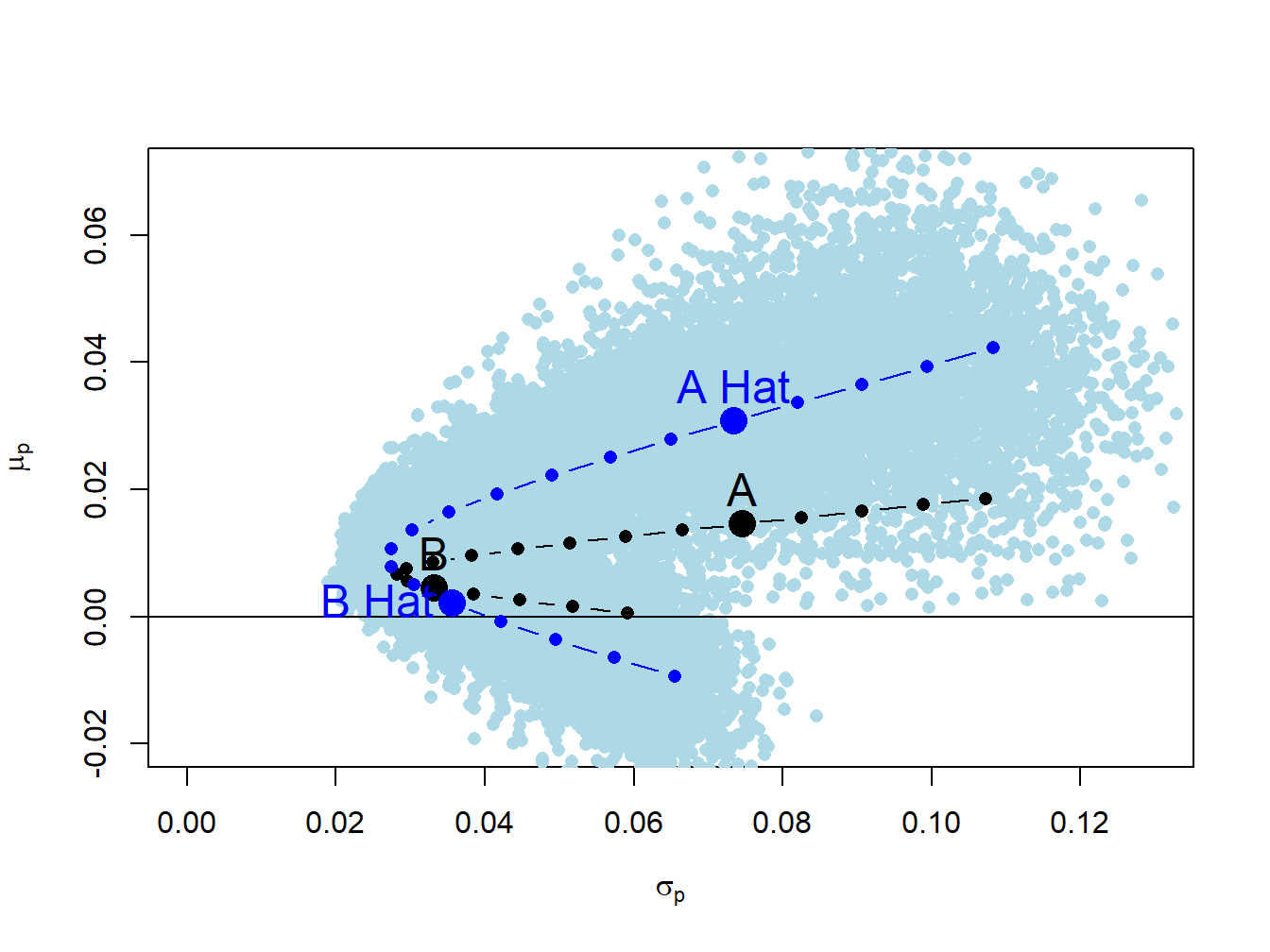
Figure 15.5: Estimated frontier with bootstrap estimates.
The true frontier portfolios are the black dots, the estimated frontier portfolios are the dark blue dots and the bootstrap risk-return pairs are the light blue dots. The bootstrap estimates form a light blue cloud around the estimated frontier. The bootstrap cloud can be interpreted as approximating a confidence interval around estimated frontier. From (15.11), this confidence interval can be thought of the union of all of the confidence ellipses about the portfolios on the frontier. The true frontier of portfolios (black dots) is within the blue cloud.
\(\blacksquare\)
15.1.2 Statistical properties of the global minimum variance portfolio
For portfolios of two risky assets, the global minimum variance portfolio weights satisfy \[\begin{equation} x_{A}^{\min}=\frac{\sigma_{B}^{2}-\sigma_{AB}}{\sigma_{A}^{2}+\sigma_{B}^{2}-2\sigma_{AB}},~x_{B}^{\min}=1-x_{A}^{\min}=\frac{\sigma_{A}^{2}-\sigma_{AB}}{\sigma_{A}^{2}+\sigma_{B}^{2}-2\sigma_{AB}}.\tag{15.12} \end{equation}\] The expected return and variance of the global minimum variance portfolio are \[\begin{eqnarray*} \mu_{p,\mathrm{min}} & = & x_{A}^{\mathrm{min}}\mu_{A}+x_{B}^{\mathrm{min}}\mu_{B},\\ \sigma_{p,\mathrm{min}}^{2} & = & \left(x_{A}^{\mathrm{min}}\right)^{2}\sigma_{A}^{2}+\left(x_{B}^{\mathrm{min}}\right)^{2}\sigma_{B}^{2}+2x_{A}^{\mathrm{min}}x_{B}^{\mathrm{min}}\sigma_{AB}. \end{eqnarray*}\]
The estimated global minimum variance portfolio weights are then \[\begin{equation} \hat{x}_{A}^{\min}=\frac{\hat{\sigma}_{B}^{2}-\hat{\sigma}_{AB}}{\hat{\sigma}_{A}^{2}+\hat{\sigma}{}_{B}^{2}-2\hat{\sigma}_{AB}},~x_{B}^{\min}=1-\hat{x}{}_{A}^{\min}=\frac{\hat{\sigma}{}_{A}^{2}-\hat{\sigma}{}_{AB}}{\hat{\sigma}_{A}^{2}+\hat{\sigma}_{B}^{2}-2\hat{\sigma}{}_{AB}}.\tag{15.13} \end{equation}\] From (15.13) we see that estimation error in the global minimum variance weights is related to estimation error in the asset variances and the covariance in a complicated nonlinear way. However, the estimation error does not depend on estimation error in the expected returns. The estimated expected returns and variance of the global minimum variance portfolio are \[\begin{eqnarray} \hat{\mu}_{p,\mathrm{min}} & = & \hat{x}{}_{A}^{\mathrm{min}}\hat{\mu}_{A}+\hat{x}{}_{B}^{\mathrm{min}}\hat{\mu}_{B},\tag{15.14}\\ \hat{\sigma}_{p,\mathrm{min}}^{2} & = & \left(\hat{x}{}_{A}^{\mathrm{min}}\right)^{2}\hat{\sigma}_{A}^{2}+\left(\hat{x}{}_{B}^{\mathrm{min}}\right)^{2}\hat{\sigma}_{B}^{2}+2\hat{x}{}_{A}^{\mathrm{min}}\hat{x}_{B}^{\mathrm{min}}\hat{\sigma}_{AB}\tag{15.15} \end{eqnarray}\] Here, estimation error in \(\hat{\mu}_{p,\mathrm{min}}\) depends on two sources: estimation error in the global minimum variance weights (which depend on estimation error in the asset variances and the covariance), and estimation error in the asset expected returns. However, estimation error in \(\hat{\sigma}_{p,\mathrm{min}}^{2}\) only depends on estimation error in the asset variances and the covariance. Because there is more estimation error in the asset expected returns than the asset variances \(\hat{\mu}_{p,\mathrm{min}}\), will be estimated more imprecisely than \(\hat{\sigma}_{p,\mathrm{min}}^{2}\).
For the example data, the true and estimated global minimum variance portfolio are:
# True global min variance portfolio weights
xA.min = (sig2.B - sig.AB)/(sig2.A + sig2.B - 2*sig.AB)
xB.min = 1 - xA.min
c(xA.min, xB.min)
## [1] 0.2020859 0.7979141# Estimated min variance portfolio weights
xA.min.hat = (sig2hat.vals[2] - covhat)/
(sig2hat.vals[1] + sig2hat.vals[2] - 2*covhat)
xB.min.hat = 1 - xA.min.hat
c(xA.min.hat, xB.min.hat)## asset.B asset.B
## 0.2530985 0.7469015The estimated weights are close to the true weights. The true and estimated expected return and volatility of the global minimum variance portfolio are:
# Expected return and volatility of true global minimum variance portfolio
mu.p.min = xA.min*mu.A + xB.min*mu.B
sig2.p.min = xA.min^2 * sig2.A + xB.min^2 * sig2.B +
               2*xA.min*xB.min*sig.AB
sig.p.min = sqrt(sig2.p.min)
c(mu.p.min, sig.p.min)
## [1] 0.006604192 0.028238698# Expected return and volatility of estimated global
# minimum variance portfolio
mu.p.min.hat = as.numeric(xA.min.hat*muhat.vals[1] +
xB.min.hat*muhat.vals[2])
sig2.p.min.hat = xA.min.hat^2 * sig2hat.vals[1] +
xB.min.hat^2 * sig2hat.vals[2] +
2*xA.min.hat*xB.min.hat*covhat
sig.p.min.hat = as.numeric(sqrt(sig2.p.min.hat))
c(mu.p.min.hat, sig.p.min.hat)## [1] 0.009370107 0.027055059The estimated volatility of the global minimum variance portfolio is close to the true volatility but the estimated expected return is much larger than the true expected return. These portfolios are illustrated in Figure 15.6.
\(\blacksquare\)
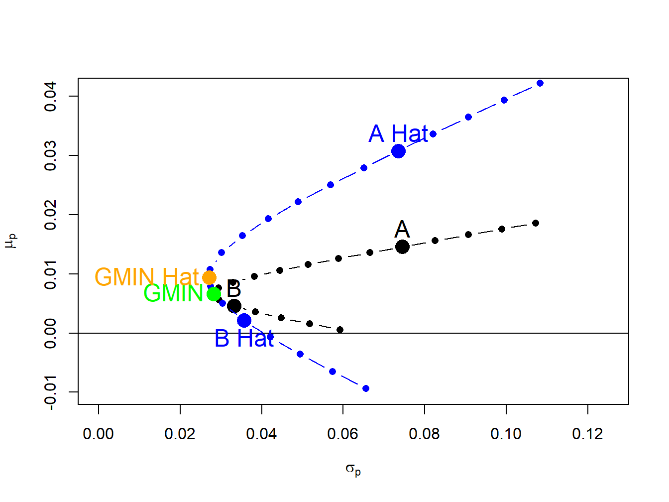
Figure 15.6: True and estimated global minimum variance portfolios.
The statistical properties of (15.13), (15.14) and (15.15) are difficult to derive analytically. For example, suppose we would like to evaluate the bias in the global minimum variance weights. We would need to evaluate \[\begin{equation} E\left[\hat{x}_{A}^{\min}\right]=E\left[\frac{\hat{\sigma}_{B}^{2}-\hat{\sigma}_{AB}}{\hat{\sigma}_{A}^{2}+\hat{\sigma}{}_{B}^{2}-2\hat{\sigma}_{AB}}\right].\tag{15.16} \end{equation}\] Now, \[ E\left[\frac{\hat{\sigma}_{B}^{2}-\hat{\sigma}_{AB}}{\hat{\sigma}_{A}^{2}+\hat{\sigma}{}_{B}^{2}-2\hat{\sigma}_{AB}}\right]\neq\frac{E\left[\hat{\sigma}_{B}^{2}\right]-E\left[\hat{\sigma}_{AB}\right]}{E\left[\hat{\sigma}_{A}^{2}\right]+E\left[\hat{\sigma}{}_{B}^{2}\right]-2E\left[\hat{\sigma}_{AB}\right]} \] because \(E[g(X)]\neq g(E[X])\) for nonlinear functions \(g(\cdot)\). Hence, (15.16) is extremely difficult to evaluate analytically. Similarly, suppose we would like to compute \(\mathrm{se}(\hat{x}_{A}^{\min}).\) We would need to compute \[ \mathrm{var}\left(\hat{x}_{A}^{\min}\right)=\mathrm{var}\left(\frac{\hat{\sigma}_{B}^{2}-\hat{\sigma}_{AB}}{\hat{\sigma}_{A}^{2}+\hat{\sigma}{}_{B}^{2}-2\hat{\sigma}_{AB}}\right), \] which is a difficult and tedious calculation and can only be approximated based on the CLT.
The computations are even more difficult for evaluating bias and computing standard errors for (15.14) and (15.15). For example, to evaluate the bias of \(\hat{\mu}_{p,\mathrm{min}}\) we need to calculate \[\begin{equation} E\left[\hat{\mu}_{p,\mathrm{min}}\right]=E\left[\hat{x}{}_{A}^{\mathrm{min}}\hat{\mu}_{A}+\hat{x}{}_{B}^{\mathrm{min}}\hat{\mu}_{B}\right]=E\left[\hat{x}{}_{A}^{\mathrm{min}}\hat{\mu}_{A}\right]+E\left[\hat{x}{}_{B}^{\mathrm{min}}\hat{\mu}_{B}\right].\tag{15.17} \end{equation}\] Without knowing more about the joint distributions of the asset means and weights we cannot simplify (15.17). To compute the standard error of \(\hat{\mu}_{p,\mathrm{min}}\) we need to calculate \[\begin{align*} \mathrm{var}\left(\hat{\mu}_{p,\mathrm{min}}\right)&=\mathrm{var}\left(\hat{x}{}_{A}^{\mathrm{min}}\hat{\mu}_{A}+\hat{x}{}_{B}^{\mathrm{min}}\hat{\mu}_{B}\right)\\ &=\mathrm{var}(\hat{x}{}_{A}^{\mathrm{min}}\hat{\mu}_{A})+\mathrm{var}(\hat{x}{}_{B}^{\mathrm{min}}\hat{\mu}_{B})+2\mathrm{cov}\left(\hat{x}{}_{A}^{\mathrm{min}}\hat{\mu}_{A},\,\hat{x}{}_{B}^{\mathrm{min}}\hat{\mu}_{B}\right). \end{align*}\]
Again, without knowing more about the joint distributions of the asset means and estimated weights we cannot simplify (15.17).
Fortunately, statistical properties of (15.13), (15.14) and (15.15) can be easily quantified using the bootstrap. For each bootstrap sample we calculate these statisticss and from the bootstrap distributions we can then evaluate bias and compute standard errors and confidence intervals.
To compute \(B=1000\) bootstrap estimates of (15.13), (15.14) and (15.15) use:
# initialize matrices
n.boot = 1000
weights.boot = matrix(0, n.boot, 2)
stats.boot = matrix(0, n.boot, 2)
colnames(weights.boot) = names(mu.vec)
colnames(stats.boot) = c("mu", "sigma")
# bootstrap loop
set.seed(123)
for (i in 1:n.boot) {
   boot.idx = sample(n.obs, replace=TRUE)
   ret.boot = returns.sim[boot.idx, ]
# CER model estimates
   muhat.boot = colMeans(ret.boot)
   sig2hat.boot = apply(ret.boot, 2, var)
   sigmahat.boot = sqrt(sig2hat.boot)
   covhat.boot = cov(ret.boot)[1,2]
# global minimum variance portfolio weights
   weights.boot[i, 1] = (sig2hat.boot[2] - covhat.boot)/
                        (sig2hat.boot[1] + sig2hat.boot[2] -
                            2*covhat.boot)
   weights.boot[i, 2] = 1 - weights.boot[i, 1]
# portfolio risk return estimates
   stats.boot[i, "mu"] = weights.boot[i, 1]*muhat.boot[1] +
                         weights.boot[i, 2]*muhat.boot[2]
   sig2.boot = (weights.boot[i, 1]^2 * sig2hat.boot[1] +
                weights.boot[i, 2]^2 * sig2hat.boot[2]
                + 2*weights.boot[i, 1]*weights.boot[i, 2]*covhat.boot)
   stats.boot[i, "sigma"] = sqrt(sig2.boot)
}
The bootstrap bias estimates for the global minimum variance portfolio weights are:
##       asset.A       asset.B
##  0.0008862438 -0.0008862438
These values are close to zero suggesting that the estimated weights are unbiased. Notice that the estimates are identical but opposite in sign. This arises because the bootstrap estimates are perfectly negatively correlated:
## [1] -1The bootstrap standard error estimates for the weights are:
##    asset.A    asset.B
## 0.04538304 0.04538304
The standard errors estimates are identical and close to 0.05 which is not too large. Figure 15.7 shows histograms and normal QQ-plots for the bootstrap estimates of the weights. These distributions are centered at the sample estimates (white vertical lines) and look slightly asymmetric.
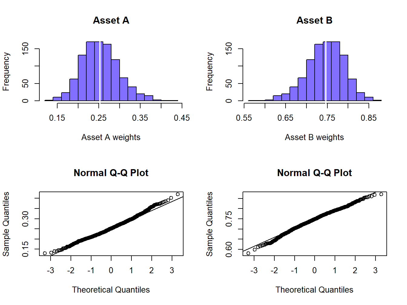
Figure 15.7: Empirical distribution of bootstrap estimates of global minimum variance portfolio weights.
The bootstrap estimates of bias for the estimated expected return and volatility of the global minimum variance portfolio are:
##            mu         sigma
##  0.0003824980 -0.0006440685
These small values indicate that the estimates are roughly unbiased. The bootstrap standard error estimates are:
##          mu       sigma
## 0.003450625 0.002336063
Here, the bootstrap standard error estimate for \(\hat{\mu}_{p,\mathrm{min}}\) is larger than the estimate for \(\hat{\sigma}_{p,\mathrm{min}}\) indicating more uncertainty about the mean of the global minimum variance portfolio than the volatility of the portfolio. Interestingly, the bootstrap standard error estimates are close to the naive analytical standard error formulas based on the CLT that ignore estimation error in the weights:
## [1] 0.003492793## [1] 0.002469778That is, \[ \mathrm{se_{boot}}(\hat{\mu}_{p,\mathrm{min}})\approx\frac{\hat{\sigma}_{p,\mathrm{min}}}{\sqrt{T}},\,\mathrm{se_{boot}}\left(\hat{\sigma}_{p,\mathrm{min}}\right)\approx\frac{\hat{\sigma}_{p,\mathrm{min}}}{\sqrt{2\cdot T}}. \] The histograms and normal QQ-plots of the bootstrap estimates of \(\mu_{p,min}\) and \(\sigma_{p,min}\) are illustrated in Figure 15.8, and look like normal distributions.
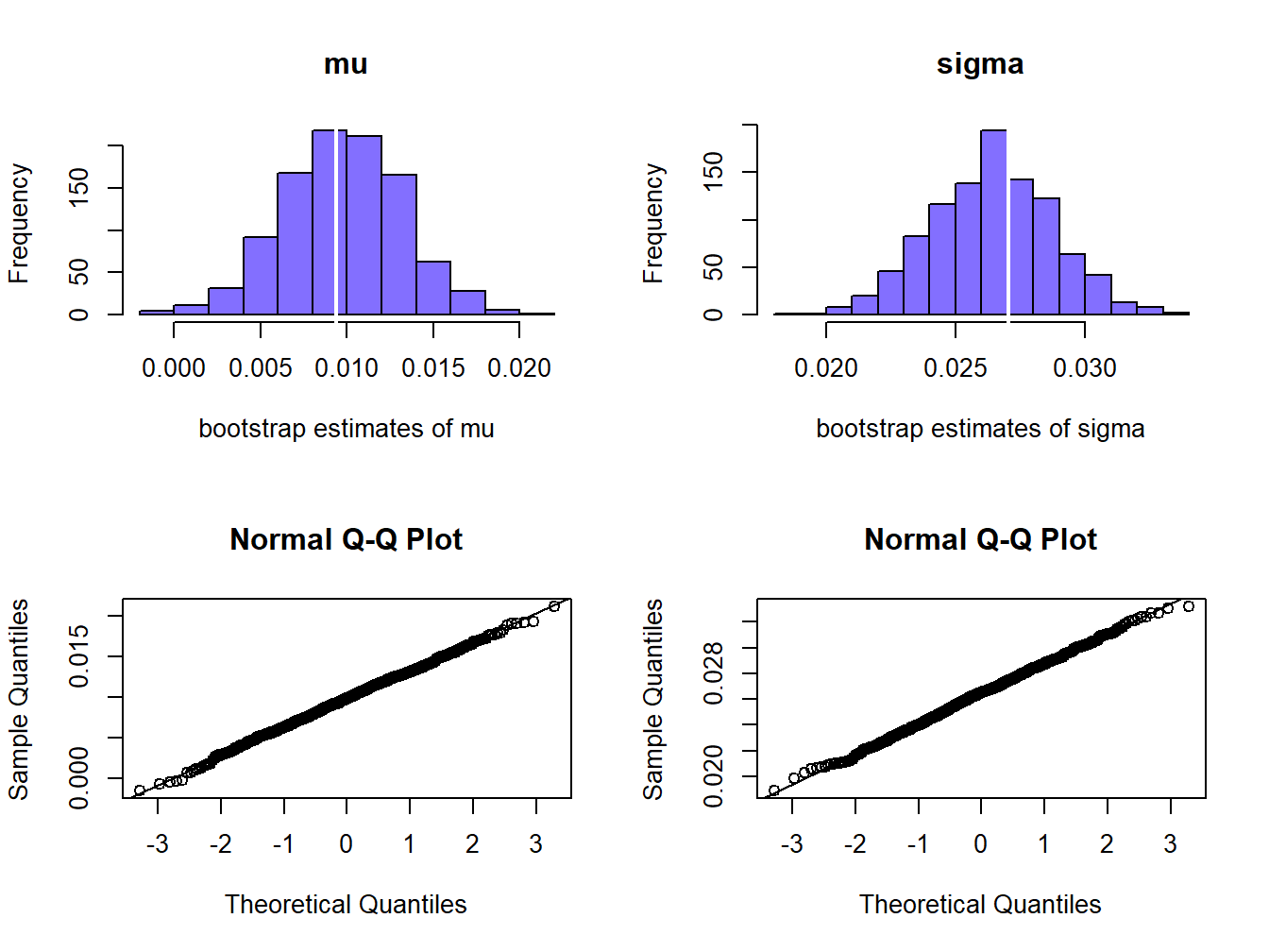
Figure 15.8: Empirical distribution of bootstrap estimates of \(\mu_{p,min}\) and \(\sigma_{p,min}\).
The sampling uncertainty in \(\hat{\mu}_{p,\mathrm{min}}\) and \(\hat{\sigma}_{p,\mathrm{min}}\) can be visualized by plotting the bootstrap estimates of \(\mu_{p,min}\) and \(\sigma_{p,min}\) on the risk return diagram, as shown in Figure 15.9. Clearly there is much more uncertainty about the location of \(\mu_{p,min}\) than the location of \(\sigma_{p,min}\) .
\(\blacksquare\)
To sum up, for the global minimum variance portfolio we have roughly unbiased estimates of the weights, expected return and variance. We have a fairly precise estimate of volatility but an imprecise estimate of expected return.
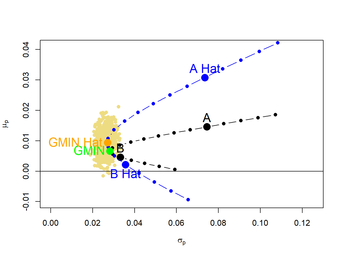
Figure 15.9: Estimation error in estimates of the global minimum variance portfolio.
15.1.3 Statistical properties of the Sharpe ratio and the tangency portfolio
Let \(r_{f}\) denote the rate of return on a risk free asset with maturity equal to the investment horizon of the return \(R_{i}\) on risky asset \(i\). Recall from chapter 11, the Shapre ratio of asset \(i\) is defined as \[ \mathrm{S}\mathrm{R}_{i}=\frac{\mu_{i}-r_{f}}{\sigma_{i}}, \] and is a measure of risk-adjusted expected return. Graphically in the risk-return diagram, \(\mathrm{S}\mathrm{R}_{i}\) is the slope of a straight line from the risk-free rate that passes through the point \((\sigma_{i},\mu_{i})\) and represents the risk-return tradeoff of portfolios of the risk-free asset and the risky asset. The estimated Sharpe ratio is \[ \widehat{\mathrm{SR}}_{i}=\frac{\hat{\mu}_{i}-r_{f}}{\hat{\sigma}_{i}}, \] which inherits estimation error from \(\hat{\mu}_{i}\) and \(\hat{\sigma}_{i}\) in a nonlinear way. As a result, analytically computing the bias and standard error for \(\widehat{\mathrm{SR}}_{i}\) is complicated and typically involves approximations based on the CLT. However, computing numerical estimates of the bias and the standard error for \(\widehat{\mathrm{SR}}_{i}\) using the bootstrap is simple.
For the example data, assume a monthly risk-free rate of \(r_{f}=0.03/12=0.0025.\) The true Sharpe ratios are:
##    asset.A    asset.B
## 0.16223990 0.06275546
Here, asset A has a much higher Sharpe ratio than asset B. For the simulated data, the estimated Sharpe ratios are:
##    asset.A    asset.B
##  0.3849417 -0.0107315
For both assets the estimated Sharpe ratios are quite different from the true Sharpe ratios and are highly misleading. The estimated Sharpe ratio for asset A is more than two times larger than the true Sharpe ratio and indicates a much higher risk adjusted preformance than is actually available. For asset B, the estimated Sharpe ratio is slightly negative when, in fact, the true Sharpe ratio is slightly positive. The true and estimated Sharpe ratios are illustrated in Figure 15.10. The slopes of the black lines are the true Sharpe ratios, and the slopes of the blues lines are the estimated Sharpe ratios.
\(\blacksquare\)
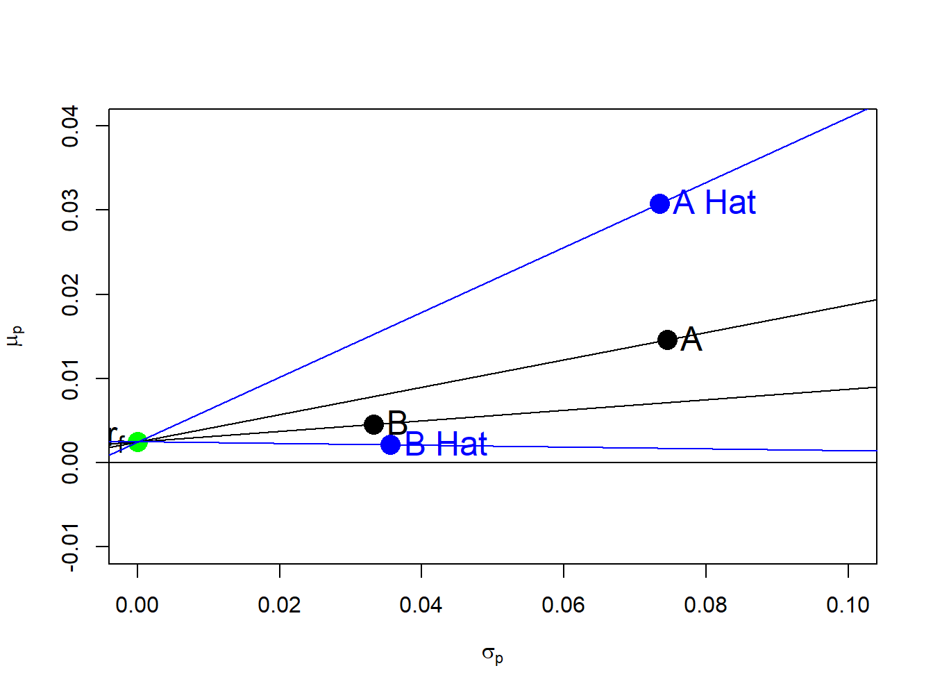
Figure 15.10: True and estimated Sharpe ratios.
To illustrate the magnitude of the estimation errors in the estimated Sharpe ratios, Figure 15.11 shows 500 bootstrap estimates of the risk-return pairs \((\sigma_{A},\mu_{A})\) and \((\sigma_{B},\mu_{B})\) along with the maximum and minimum bootstrap Sharpe ratio estimates for each asset. The bootstrap Sharpe ratio estimates are computed using:
n.boot = 500
mu.boot = matrix(0, n.boot, 2)
sd.boot = matrix(0, n.boot, 2)
SR.boot = matrix(0, n.boot, 2)
colnames(mu.boot) = colnames(sd.boot) = colnames(SR.boot) = c("A", "B")
set.seed(123)
for (i in 1:n.boot) {
   boot.idx = sample(n.obs, replace=TRUE)
   ret.boot = returns.sim[boot.idx, ]
   mu.boot[i, ] = colMeans(ret.boot)
   sd.boot[i, ] = apply(ret.boot, 2, sd)
   SR.boot[i, ] = (mu.boot[i, ] - r.f)/sd.boot[i, ]
}
# find index of max and min bootstrap Sharpe ratios
maxSRidx.A = which(SR.boot[, 1] == max(SR.boot[, 1]))
minSRidx.A = which(SR.boot[, 1] == min(SR.boot[, 1]))
maxSRidx.B = which(SR.boot[, 2] == max(SR.boot[, 2]))
minSRidx.B = which(SR.boot[, 2] == min(SR.boot[, 2]))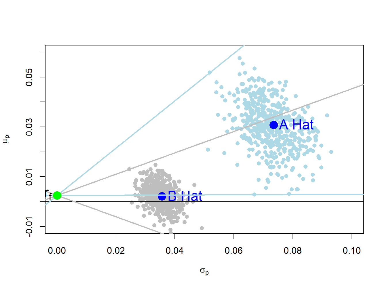
Figure 15.11: Bootstrap risk-return estimates with maximum and minimum Sharpe ratios.
The maximum and minimum bootstrap Sharpe ratio estimates for asset B are the two grey straight lines from the risk-free rate that have the highest and lowest slopes, respectively. The maximum and minimum bootstrap Sharpe ratio estimates for asset A are the two light blue lines with the highest and lowest slopes, respectively. These maximum and minimum estimates are:
##         A         B
## 0.9516121 0.4291045## A B
## 0.004672635 -0.429456951For each asset the difference in the maximum and minimum slopes is substantial and indicates a large about of estimation error in the estimated Sharpe ratios.
The statistical properties of the estimated Sharpe ratios can be estimated from the bootstrap samples. The bootstrap estimates of bias are:
##           A           B
## 0.23161575 -0.06416556## A B
## 1.427613 -1.022470Here we see there is a substantial upward bias in \(\widehat{\mathrm{SR}}_{A}\) (bias relative to true Sharpe ratio is 141%) and a substantial downward bias in \(\widehat{\mathrm{SR}}_{B}\) (bias relative to true Sharpe ratio is -105%). A crude bias adjusted Sharpe ratio estimate, which substracts the estimated bias from the sample estimate, gives results much closer to the true Sharpe ratios:
##    asset.A    asset.B
## 0.15332595 0.05343406## asset.A asset.B
## 0.16223990 0.06275546The bootstrap estimated standard errors for both assets are big and indicate that the Sharpe ratios are not estimated well:
##         A         B
## 0.1541520 0.1320264
Figure 15.12 shows the histograms and normal QQ-plots of the bootstrap distributions for the estimated Sharpe ratios. The histograms for both assets show the wide dispersion of the bootstrap Sharpe ratio estimates that was illustrated in Figure 15.11. The histogram and QQ-plot for asset A shows a positive skewness whereas the histogram and QQ-plot for asset B show a more symmetric distribution. The quantile-based 95% confidence intervals for the true Sharpe ratios are:
##      2.5%     97.5%
## 0.0963779 0.7093436## 2.5% 97.5%
## -0.2606848 0.2630487These intervals are quite large and indicate much uncertainty about the true Sharpe ratio values.
\(\blacksquare\)
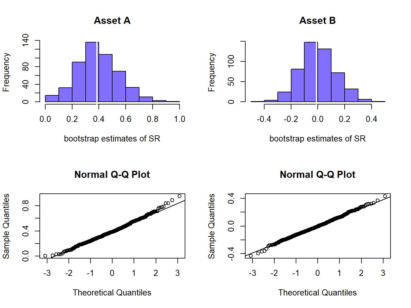
Figure 15.12: Bootstrap distributions of estimated Sharpe ratios.
\(\hat{\sigma}_{i}\) is asymptotically unbiased and the bias for finite \(T\) is typically very small so that it is essentially unbiased for moderately sized \(T\).↩︎
Notice, however, that the pair \((\sigma_{p},\mu_{p})\) is inside the confidence ellipse for \((\sigma_{B},\mu_{B})\) but that \((\sigma_{B},\mu_{B})\) is not in the confidence ellipse for \((\sigma_{p},\mu_{p})\). ↩︎