8.7 Using Monte Carlo Simulation to Evaluate Delta Method, Jackknife and Bootstrap Standard Errors
we have studied three ways of computing standard errors for functions of GWN model parameters
Give similar resuts for the example functions
What are the preferred methods in practice?
Which methods are most accurate?
Use MC Simulation to evaluate the three methods in stylized model in which the GWN model is true. MC can give the best numerical standard error with which we can compare to the delta method, jackknife and bootstrap standard errors.
We can evaluate the statistical properties of \(f_j(\hat{\theta})\), for \(j=1,\ldots,4\), by Monte Carlo simulation in the same way that we evaluated the statistical properties of \(\hat{\mu}\) in Chapter 7.We use the simulation model (7.41) and \(N=1000\) simulated samples of size \(T=100\) to compute the estimates \(\{\left(f_{j}(\hat{\theta})\right)^{1},\ldots,\left(f_j(\hat{\theta})\right)^{1000}\}\) The true values for \(f_j(\theta)\) are: \[\begin{align*} f_1(\theta) & = 0.05+(0.10)\times(-1.645)=-0.114,\\ f_2(\theta) & = - \$100,000 \times f_1(\theta) = \$11,449, \\ f_3(\theta) & = \$100,000 \times \left(\exp(f_1(\theta)) -1 \right) = \$10,818, \\ f_4(\theta) & = (0.05 - 0.0025)/0.10 = 0.475. \end{align*}\]
The R code for the simulation loop is:
mu = 0.05
sigma = 0.10
W0 = 100000
r.f = 0.0025
f1 = mu + sigma*qnorm(0.05)
f2 = -W0*f1
f3 = -W0*(exp(f1) - 1)
f4 = (mu - r.f)/sigma
n.obs = 172
n.sim = 1000
set.seed(111)
sim.f = matrix(0,n.sim,4)
dm.f = matrix(0, n.sim, 4)
jack.f = matrix(0, n.sim, 4)
boot.f = matrix(0, n.sim, 4)
boot.bias = matrix(0, n.sim, 4)
colnames(sim.f) = colnames(dm.f) = colnames(jack.f) = c("f1", "f2","f3","f4")
colnames(boot.f) = colnames(boot.bias) = c("f1", "f2","f3","f4")

for (sim in 1:n.sim) {
sim.ret = rnorm(n.obs,mean=mu,sd=sigma)
muhat = mean(sim.ret)
sigmahat = sd(sim.ret)
sim.f[sim, "f1"] = muhat + sigmahat*qnorm(0.05)
sim.f[sim, "f2"] = -W0*sim.f[sim, "f1"]
sim.f[sim, "f3"] = -W0*(exp(sim.f[sim, "f1"]) - 1)
sim.f[sim, "f4"] = (muhat - r.f)/sigmahat
# delta method se
dm.f[sim, "f1"] = (sigmahat/sqrt(n.obs))*sqrt(1 + 0.5*qnorm(0.05)^2)
dm.f[sim, "f2"] = W0*dm.f[sim, "f1"]
dm.f[sim, "f3"] = W0*exp(sim.f[sim, "f1"])*dm.f[sim, "f1"]
dm.f[sim, "f4"] = sqrt((1/n.obs)*(1 + 0.5*(sim.f[sim, "f4"]^2)))
# jackknife se
f1.jack = jackknife(1:n.obs, theta=theta.f1, as.matrix(sim.ret))
jack.f[sim, "f1"] = f1.jack$jack.se
f2.jack = jackknife(1:n.obs, theta=theta.f2, as.matrix(sim.ret), W0)
jack.f[sim, "f2"] = f2.jack$jack.se
f3.jack = jackknife(1:n.obs, theta=theta.f3, as.matrix(sim.ret), W0)
jack.f[sim, "f3"] = f3.jack$jack.se
f4.jack = jackknife(1:n.obs, theta=theta.f4, as.matrix(sim.ret), r.f)
jack.f[sim, "f4"] = f4.jack$jack.se
# bootstrap se
f1.bs = boot(sim.ret, statistic = f1.boot, R=999)
boot.f[sim, "f1"] = sd(f1.bs$t)
f2.bs = boot(sim.ret, statistic = f2.boot, R=999)
boot.f[sim, "f2"] = sd(f2.bs$t)
f3.bs = boot(sim.ret, statistic = f3.boot, R=999)
boot.f[sim, "f3"] = sd(f3.bs$t)
f4.bs = boot(sim.ret, statistic = f4.boot, R=999)
boot.f[sim, "f4"] = sd(f4.bs$t)
# bootstrap bias
boot.bias[sim, "f1"] = summary(f1.bs)$bootBias
boot.bias[sim, "f2"] = summary(f2.bs)$bootBias
boot.bias[sim, "f3"] = summary(f3.bs)$bootBias
boot.bias[sim, "f4"] = summary(f4.bs)$bootBias
}
The histograms of \(f_j(\hat{\theta})\) values are displayed in Figure 8.5. The dotted white lines indicate the true values, \(f_j(\theta)\).
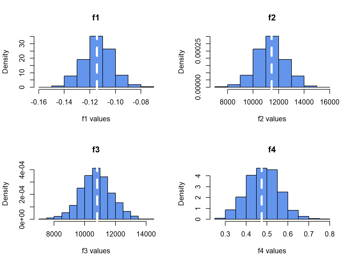
Figure 8.5: Histograms of \(\hat{f}_{j}\) (for \(j=1,\ldots, 4\)) computed from \(N=1000\) Monte Carlo samples from the GWN model.
The histograms for the \(f_j(\hat{\theta})\) values are bell-shaped for \(j=1,2,3\) and the histogram for \(j=4\) is slightly right skewed. All of the histograms are centered very close to the respective true values. Recall, the standard deviation of the Monte Carlo estimates (spread of the histograms about true value) approximates the true standard error of the plug-in estimates.
The Monte Carlo estimates of bias are:
##      f1      f2      f3      f4
##   0.001 -72.910 -70.920   0.007
which confirm that \(f_j\) are essentially unbiased estimators. It is often useful to also look at the bias relative to the true value to eliminate units:
##       f1       f2       f3       f4
## -0.00637 -0.00637 -0.00656  0.01454
In relative terms, the largest bias is 1.45%, which occurs for the estimate of the Sharpe ratio.
The average bootstrap estimate of bias is:
##      f1      f2      f3      f4
##   0.001 -71.824 -70.213   0.003
The bootstrap bias values are very close to the Monte Carlo estimates of bias which indicates that the bootstrap estimate of bias is very accruate in this context.
The sample standard deviations of the Monte Carlo estimates approximate the true standard errors of the estimated functions:
##       f1       f2       f3       f4
##    0.011 1147.869 1024.379    0.078
The sample means of the delta method, jackknife, and bootstrap standard errors give the average performance of these estimated standard errors. It is informative to compare these average standard errors to the Monte Carlo standard errors:
dm.se = colMeans(dm.f)
jack.se = colMeans(jack.f)
boot.se = colMeans(boot.f)
ans = rbind(dm.se/mc.se, jack.se/mc.se, boot.se/mc.se)
rownames(ans) = c("Delta Method", "Jackknife", "Bootstrap")
ans
## f1 f2 f3 f4
## Delta Method 1.02 1.02 1.02 1.03
## Jackknife 1.01 1.01 1.01 1.04
## Bootstrap 1.00 1.00 1.00 1.04In the table above, a value of \(1\) means the estimated standard error is the same as the Monte Carlo standard error (on average), and a value greater than \(1\) means that the estimated standard error is larger than the Monte Carlo standard error (on average). Here, we see that all of the estimated standard errors are very close to the Monte Carlo standard errors, and overall the bootstrap estimated standard errors are the closest. The worst performance is for \(f_4(\hat{\theta})\) where the estimated standard errors are about 3% to 4% larger than the Monte Carlo standard errors.
It is also useful to look at the standard deviations of the estimated standard errors over the Monte Carlo simulations. This tells us how variable the estimated standard errors are across different simulations:
dm.sd = apply(dm.f,2,sd)
jack.sd = apply(jack.f,2,sd)
boot.sd = apply(boot.f,2,sd)
ans = rbind(dm.sd, jack.sd, boot.sd)
rownames(ans) = c("Delta Method", "Jackknife", "Bootstrap")
ans
## f1 f2 f3 f4
## Delta Method 0.000654 65.4 49.8 0.00137
## Jackknife 0.001158 115.8 98.7 0.00365
## Bootstrap 0.001163 115.2 98.5 0.00406Here, we see that, across the simulations, the delta method is the least variable and the jackknife and the bootstrap have similar variability that is about twice as large as the delta method variability. The variability of the bootstrap can be reduced by increasing the number of bootstrap simulations (here it is 1000).
Overall, the Monte Carlo experiment confirms that the delta method, jackknife and bootstrap all produce accurate standard error estimates for the example plug-in functions.