11.6 Application to Real World Portfolios
The portfolio theory for two risky assets and a risk-free asset developed in this chapter is not as limited as you might think if you realize that a single risky asset can also be a portfolio of many assets, such as a mutual fund of stocks or bonds, or an exchange traded fund (ETF) of stocks or bonds. In particular, a very common asset allocation for retirement portfolios is a simple two asset portfolio of in which one risky asset is a mutual fund of stocks and the other (less) risky asset is a mutual fund of U.S. Treasury bonds.
In the IntroCompFinR package there is a data object called
VanguardPrices that contains monthly adjusted closing prices
on six Vanguard mutual funds over the period January, 1995 through
December, 2014.73
The fund VFINX is a low cost fund designed to track the performance
of the S&P 500 index. The S&P 500 index is a value-weighted index of the 500 largest stocks (by market capitalization) traded on the NYSE.74 We will use this as our stock portfolio. The
fund VBLTX is a low cost fund constructed to track the performance
of a portfolio of long term (maturities greater than 10 years) U.S.
Government Bonds.75 We will use this as our bond portfolio. We will
use the U.S. 3-month T-Bill rate as the risk-free asset. The following
code creates the monthly simple return data for this example:
library(IntroCompFinR)
library(PerformanceAnalytics)
data(VanguardPrices)
VanguardPrices = as.xts(VanguardPrices)
stockBondPrices = VanguardPrices[, c("vfinx", "vbltx")]
stockBondRetS = na.omit(Return.calculate(stockBondPrices, method="simple"))
head(stockBondRetS, n=3)
## vfinx vbltx
## Feb 1995 0.0389 0.0280
## Mar 1995 0.0295 0.0102
## Apr 1995 0.0293 0.0202We will construct efficient portfolios using the GWN model estimates of expected returns, variances, and covariances over four sub-periods: January, 1995 to January 2000; January, 2000 to January, 2005; January, 2005 to January, 2010; January, 2010 to December, 2014. The approximate annualized T-Bill rates at the end of these periods are 0.05, 0.025, 0.001, and 0.001, respectively.76
# Define sub-periods
smpl1 = "1995-1::2000-1"
smpl2 = "2000-1::2005-1"
smpl3 = "2005-1::2010-1"
smpl4 = "2010-1::2014-12"
# Monthly risk-free rates for sub-periods
r.f = c(0.05, 0.025, 0.001, 0.001)/12
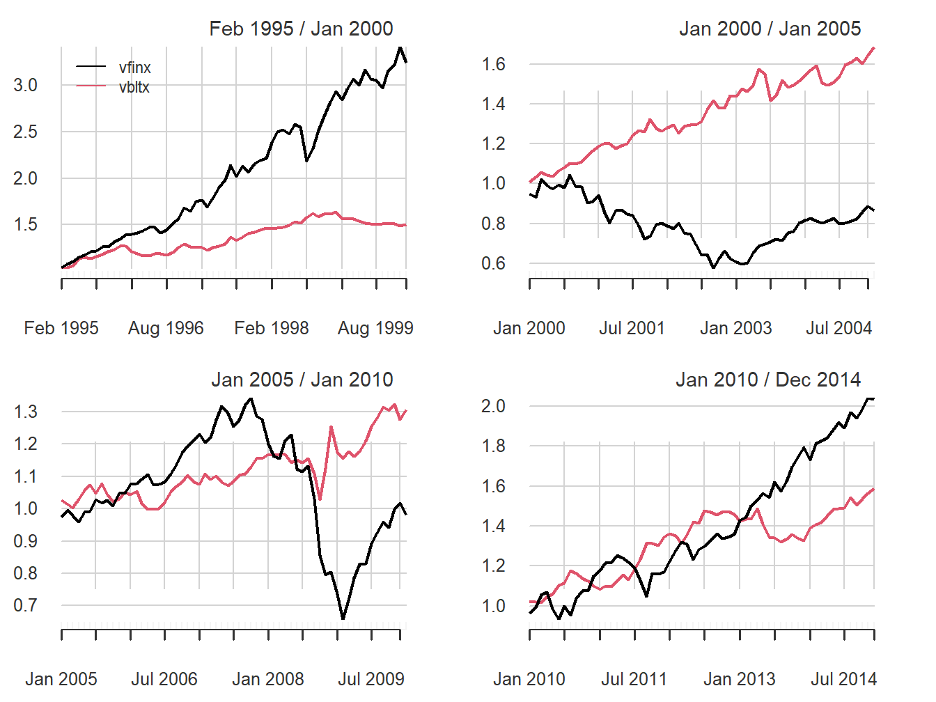
Historical performance of the stock and bond portfolios over the four sub-periods is illustrated in Figure 11.11, created using:77
par(mfrow=c(2,2))
chart.CumReturns(stockBondRetS[smpl1], main="", wealth.index = TRUE,
                 legend.loc = "topleft")
chart.CumReturns(stockBondRetS[smpl2], main="", wealth.index = TRUE)
chart.CumReturns(stockBondRetS[smpl3], main="", wealth.index = TRUE)
chart.CumReturns(stockBondRetS[smpl4], main="", wealth.index = TRUE) 
Figure 11.11: Equity curves for stock (vfinx) and bond (vbltx) portfolios over sub-periods.
The performance of stocks and bonds varies substantially over the four sub-periods. In the first and fourth sub-periods, which cover the dot-com boom and the recovery from the 2009 financial crisis, stocks substantially outperformed bonds. However, in the second and third sub-periods, which cover the dot-com bust and the 2009 financial crisis, bonds outperformed stocks.
The GWN model estimates of the monthly expected returns, volatilities,
and Sharpe ratios on the stock and bond portfolios are computed and
annualized using the square-root-of-time rule with the PerformanceAnalytics
function table.AnnualizedReturns().
# smpl1 = "1995-1::2000-1"
table.AnnualizedReturns(stockBondRetS[smpl1], Rf = r.f[1], geometric = FALSE)
## vfinx vbltx
## Annualized Return 0.248 0.0846
## Annualized Std Dev 0.143 0.0756
## Annualized Sharpe (Rf=5%) 1.381 0.4581# smpl2 = "2000-1::2005-1"
table.AnnualizedReturns(stockBondRetS[smpl2], Rf = r.f[2], geometric = FALSE) ## vfinx vbltx
## Annualized Return -0.0155 0.1069
## Annualized Std Dev 0.1628 0.0871
## Annualized Sharpe (Rf=2.5%) -0.2490 0.9399# smpl3 = "2005-1::2010-1"
table.AnnualizedReturns(stockBondRetS[smpl3], Rf = r.f[3], geometric = FALSE) ## vfinx vbltx
## Annualized Return 0.0092 0.0576
## Annualized Std Dev 0.1600 0.1021
## Annualized Sharpe (Rf=0.1%) 0.0514 0.5547# smpl4 = "2010-1::2014-12"
table.AnnualizedReturns(stockBondRetS[smpl4], Rf = r.f[4], geometric = FALSE)## vfinx vbltx
## Annualized Return 0.151 0.0965
## Annualized Std Dev 0.130 0.0864
## Annualized Sharpe (Rf=0.1%) 1.157 1.1050The annualized estimates confirm the relative performance of bonds and stocks in the four sub-periods. In general, stock returns are about twice as volatile as bond returns. Bonds performed well in all sub-periods, with annualized mean returns between 6% and 11%. In contrast, stocks only performed well in sub-periods 1 and 4 and had negative annualized mean returns in periods 2 and 3. In terms of Sharpe ratios, stocks had annualized Sharpe ratios a bit over 1 in sub-periods 1 and 4 and bonds had annualized Sharpe ratios of 0.9 and 0.55 in sub-periods 2 and 3.78
The sample correlations between the monthly stock and bond returns, by sub-period, are:
## [1] 0.2## [1] -0.185## [1] 0.24## [1] -0.435Interestingly, the estimated correlation between stocks and bonds also varies by sub-period. In sub-periods one and three, the estimated correlations are positive, and, in sub-periods two and four, the estimated correlations are negative. The observed low to negative correlation between stock and bond returns suggests good risk reduction possibilities through diversification.

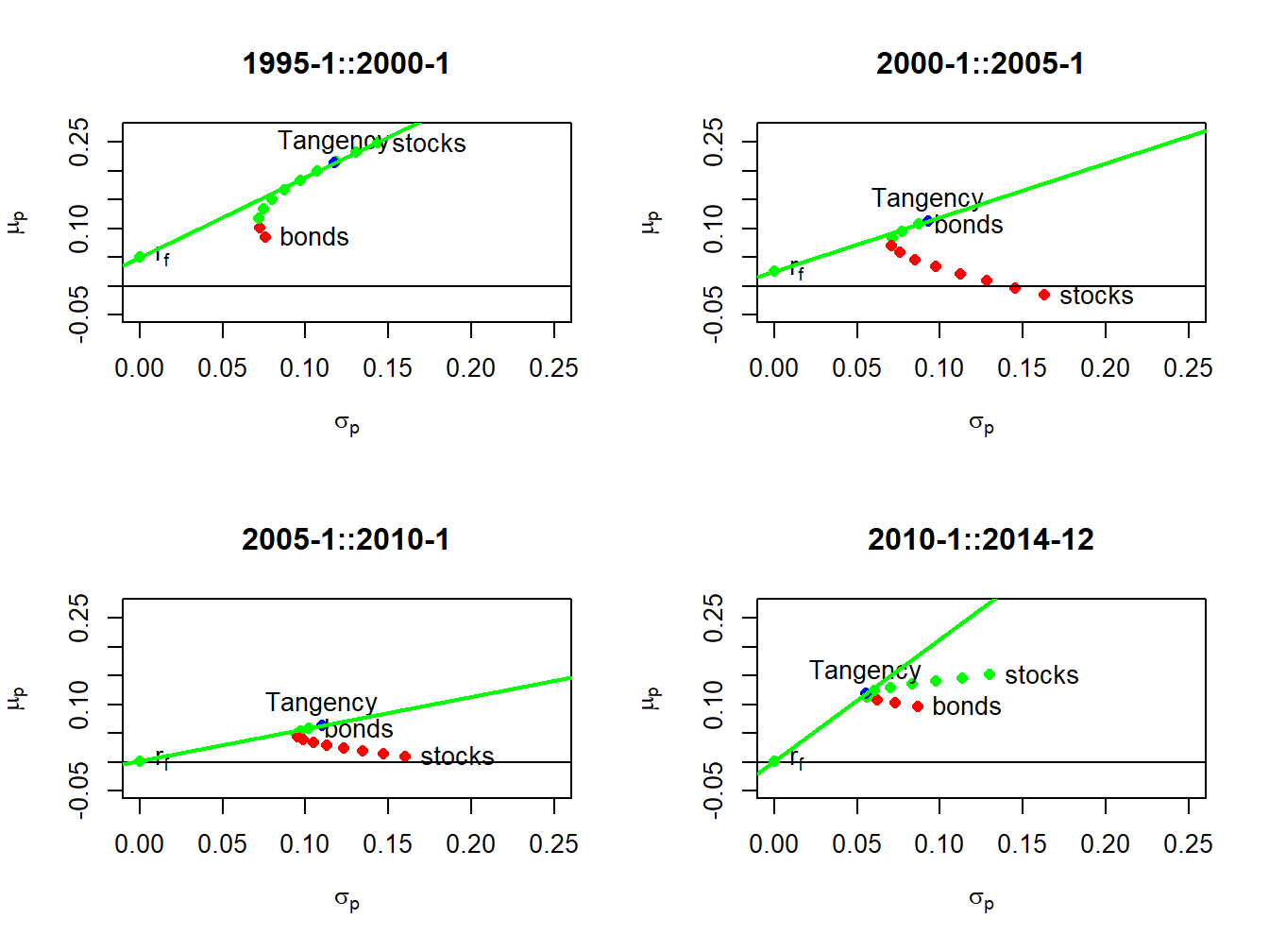
Figure 11.12: Mean-variance efficient portfolios of stocks and bonds by sub-period. Efficient portfolios are shown in green and inefficient portfolios are shown in red.
Using the sub-period GWN model estimates, we compute risky asset only efficient portfolios and efficient portfolios of T-Bills (risk-free asset) and the tangency portfolios. The resulting portfolios are illustrated in Figure 11.12. In sub-periods one and four, stocks are on the risky asset only efficient frontier and, in sub-periods two and three, bonds are on the risky asset only efficient frontier. The sub-period global minimum variance and tangency portfolios are listed in Tables 11.2 and 11.3. The global minimum variance portfolios are similar across sub-periods, with higher weights in bonds than stocks. The tangency portfolios, however, are quite different across sub-periods. In sub-periods one and four, stocks have weights 79% and 40%, respectively. In sub-periods two and three bonds essentially have 100% weights, respectively, and stocks are slighly shorted.
| \(x_{stock}\) | \(x_{bond}\) | \(\mu_{min}\) | \(\sigma_{min}\) | \(SR_{min}\) | |
|---|---|---|---|---|---|
| 1995-1::2000-1 | 0.162 | 0.838 | 0.111 | 0.072 | 0.851 |
| 2000-1::2005-1 | 0.260 | 0.740 | 0.075 | 0.070 | 0.713 |
| 2005-1::2010-1 | 0.231 | 0.769 | 0.046 | 0.094 | 0.481 |
| 2010-1::2014-12 | 0.362 | 0.638 | 0.116 | 0.055 | 2.108 |
| \(x_{stock}\) | \(x_{bond}\) | \(\mu_{tan}\) | \(\sigma_{tan}\) | \(SR_{tan}\) | |
|---|---|---|---|---|---|
| 1995-1::2000-1 | 0.789 | 0.211 | 0.213 | 0.117 | 1.393 |
| 2000-1::2005-1 | -0.047 | 1.047 | 0.113 | 0.093 | 0.943 |
| 2005-1::2010-1 | -0.107 | 1.107 | 0.063 | 0.110 | 0.561 |
| 2010-1::2014-12 | 0.404 | 0.596 | 0.119 | 0.055 | 2.128 |
This example shows the clear gains that can be made by forming efficient portfolios relative to holding stock or bonds by themselves. The results, however, are a bit misleading because the efficient portfolios formed in each sub-period use all of the data over the sub-period to estimate expected returns, volatilities, and covariances. This means that the computed efficient portfolios cannot be computed at the beginning of each sub-period. A more practical exercise would use the previous sub-period to compute GWN model estimates to be used in the subsequent sub-period. This method is explored in the end-of-chapter exercises.
Details about these funds are available at (finance.yahoo.com). ↩︎
ETF alternatives to VFINX include State Street’s SPY, Vanguard’s VOO, and iShares IVV. See
www.eft.com.↩︎ETF alternatives to VBLTX include iShares TLT and GOVT, and State Street SPTL. See
www.eft.com.↩︎Historical data on U.S. T-Bill rates is obtained from the Federal Reserve Economic Data (FRED) available at the St. Louis Fed. See
fred.stlouisfed.org↩︎The PerformanceAnalytics function
chart.CumReturns()is used to compute the equity curves for each asset.↩︎Investments with annualized Sharpe ratios greater than one are typically considered good investments.↩︎