12.5 Computing Efficient Portfolios of N risky Assets and a Risk-Free Asset Using Matrix Algebra

In Chapter 11, we showed that efficient portfolios of two risky assets and a single risk-free (T-Bill) asset are portfolios consisting of the highest Sharpe ratio portfolio (tangency portfolio) and the T-Bill. With three or more risky assets and a T-Bill the same result holds.

12.5.1 Computing the tangency portfolio using matrix algebra

The tangency portfolio is the portfolio of risky assets that has the highest Sharpe ratio. The tangency portfolio, denoted \(\mathbf{t}=(t_{\textrm{1}},\ldots,t_{N})^{\prime}\), solves the constrained maximization problem: \[\begin{equation} \underset{\mathbf{t}}{\max}~\frac{\mathbf{t}^{\prime}\mu-r_{f}}{(\mathbf{t}^{\prime}\Sigma \mathbf{t})^{{\frac{1}{2}}}}=\frac{\mu_{p,t}-r_{f}}{\sigma_{p,t}}\textrm{ s.t. }\mathbf{t}^{\prime}\mathbf{1}=1,\tag{12.25} \end{equation}\] where \(\mu_{p,t}=\mathbf{t}^{\prime}\mu\) and \(\sigma_{p,t}=(\mathbf{t}^{\prime}\Sigma \mathbf{t})^{{\frac{1}{2}}}\). The Lagrangian for this problem is: \[ L(\mathbf{t},\lambda)=\left(\mathbf{t}^{\prime}\mu-r_{f}\right)(\mathbf{t}^{\prime}\Sigma \mathbf{t})^{-{\frac{1}{2}}}+\lambda(\mathbf{t}^{\prime}\mathbf{1}-1). \] Using the chain rule, the first order conditions are: \[\begin{align*} \frac{\partial L(\mathbf{t},\lambda)}{\partial\mathbf{t}} & =\mu(\mathbf{t}^{\prime}\Sigma \mathbf{t})^{-{\frac{1}{2}}}-\left(\mathbf{t}^{\prime}\mu-r_{f}\right)(\mathbf{t}^{\prime}\Sigma \mathbf{t})^{-3/2}\Sigma \mathbf{t}+\lambda\mathbf{1}=\mathbf{0},\\ \frac{\partial L(\mathbf{t},\lambda)}{\partial\lambda} & =\mathbf{t}^{\prime}\mathbf{1}-1=0. \end{align*}\] After much tedious algebra, it can be shown that the solution for \(\mathbf{t}\) has a nice simple expression: \[\begin{equation} \mathbf{t}=\frac{\Sigma^{-1}(\mu-r_{f}\cdot\mathbf{1})}{\mathbf{1}^{\prime}\Sigma^{-1}(\mu-r_{f}\cdot\mathbf{1})}.\tag{12.26} \end{equation}\] The formula for the tangency portfolio (12.26) looks similar to the formula for the global minimum variance portfolio (12.8). Both formulas have \(\Sigma^{-1}\) in the numerator and \(\mathbf{1}^{\prime}\Sigma^{-1}\) in the denominator.

Remark

The location of the tangency portfolio, and the sign of the Sharpe ratio, depends on the relationship between the risk-free rate \(r_{f}\) and the expected return on the global minimum variance portfolio \(\mu_{p,m}\). If \(\mu_{p,m}>r_{f}\), which is the usual case, then the tangency portfolio will have a positive Sharpe ratio. If \(\mu_{p,m}<r_{f}\), which could occur when stock prices are falling and the economy is in a recession, then the tangency portfolio will have a negative Sharpe slope. In this case, efficient portfolios involve shorting the tangency portfolio and investing the proceeds in T-Bills.⁸²

Example 3.6 (Computing the tangency portfolio)

Suppose \(r_{f}=0.005\). To compute the tangency portfolio (12.26) in R for the three risky assets in Table 12.1 use:

##   MSFT   NORD   SBUX 
##  1.027 -0.326  0.299

The tangency portfolio has weights \(t_{\textrm{msft}}=1.027,\) \(t_{\textrm{nord}}=-0.326\) and \(t_{\textrm{sbux}}=0.299,\) and is given by the vector \(\mathbf{t}=(1.027,-0.326,0.299)^{\prime}.\) Notice that Nordstrom, which has the lowest mean return, is sold short in the tangency portfolio. The expected return on the tangency portfolio, \(\mu_{p,t}=\mathbf{t}^{\prime}\mu\), is:

mu.t = as.numeric(crossprod(t.vec, mu.vec))
mu.t

## [1] 0.0519

The portfolio variance, \(\sigma_{p,t}^{2}=\mathbf{t}^{\prime}\Sigma \mathbf{t}\), and standard deviation, \(\sigma_{p,t}\), are:

sig2.t = as.numeric(t(t.vec)%*%sigma.mat%*%t.vec)
sig.t = sqrt(sig2.t)
c(sig2.t, sig.t)

## [1] 0.0125 0.1116

Because \(r_{f}=0.005<\mu_{p,m}=0.0249\) the tangency portfolio has a positive Sharpe’s ratio/slope given by:

SR.t = (mu.t - r.f)/sig.t 
SR.t

## [1] 0.42

The tangency portfolio is illustrated in Figure 12.9. It is the portfolio on the efficient frontier of risky assets in which a straight line drawn from the risk-free rate to the tangency portfolio (green line) is just tangent to the efficient frontier (blue dots).

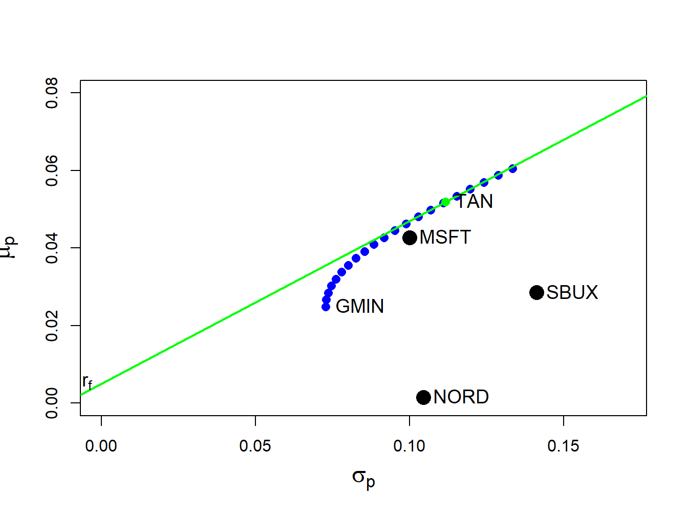
Figure 12.9: Tangency portfolio from example data.

\(\blacksquare\)

12.5.2 Alternative derivation of the tangency portfolio

The derivation of tangency portfolio formula (12.26) from the optimization problem (12.25) is a very tedious problem. It can be derived in a different way as follows. Consider forming portfolios of \(N\) risky assets with return vector \(\mathbf{R}\) and T-bills (risk-free asset) with constant return \(r_{f}\). Let \(\mathbf{x}\) denote the \(N\times1\) vector of risky asset weights and let \(x_{f}\) denote the safe asset weight and assume that \(\mathbf{x}^{\prime}\mathbf{1}+x_{f}=1\) so that all wealth is allocated to these assets. The portfolio return is: \[ R_{p,x}=\mathbf{x}^{\prime}\mathbf{R}+x_{f}r_{f}=\mathbf{x}^{\prime}\mathbf{R}+(1-\mathbf{x}^{\prime}\mathbf{1})r_{f}=r_{f}+\mathbf{x}^{\prime}(\mathbf{R}-r_{f}\cdot\mathbf{1}). \] The portfolio excess return is: \[\begin{equation} R_{p,x}-r_{f}=\mathbf{x}^{\prime}(\mathbf{R}-r_{f}\cdot\mathbf{1)}.\tag{12.27} \end{equation}\] The expected portfolio excess return (risk premium) and portfolio variance are: \[\begin{align} \mu_{p,x}-r_{f} & =\mathbf{x}^{\prime}(\mu-r_{f}\cdot\mathbf{1)},\tag{12.28}\\ \sigma_{p,x}^{2} & =\mathbf{x}^{\prime}\Sigma \mathbf{x}.\tag{11.5} \end{align}\] For notational simplicity, define \(\mathbf{\tilde{R}}=\mathbf{R}-r_{f}\cdot\mathbf{1}\), \(\tilde{\mu}=\mu-r_{f}\cdot\mathbf{1}\), \(\tilde{R}_{p,x}=R_{p,x}-r_{f}\), and \(\tilde{\mu}_{p,x}=\mu_{p,x}-r_{f}\). Then (12.27) and (12.28) can be re-expressed as: \[\begin{align} \tilde{R}_{p,x} & =\mathbf{x}^{\prime}\tilde{\mathbf{R}},\tag{12.29}\\ \tilde{\mu}_{p,x} & =\mathbf{x}^{\prime}\tilde{\mu}.\tag{12.30} \end{align}\] To find the minimum variance portfolio of risky assets and a risk free asset that achieves the target excess return \(\tilde{\mu}_{p,0}=\mu_{p,0}-r_{f}\) we solve the minimization problem: \[ \min_{\mathbf{x}}~\sigma_{p,x}^{2}=\mathbf{x}^{\prime}\Sigma \mathbf{x}\textrm{ s.t. }\tilde{\mu}_{p,x}=\tilde{\mu}_{p,0}. \] Note that \(\mathbf{x}^{\prime}\mathbf{1}=1\) is not a constraint because wealth need not all be allocated to the risky assets; some wealth may be held in the riskless asset. The Lagrangian is: \[ L(\mathbf{x},\lambda)=\mathbf{x}^{\prime}\mathbf{\Sigma x+}\lambda\mathbf{(x}^{\prime}\tilde{\mu}-\tilde{\mu}_{p,0}). \] The first order conditions for a minimum are: \[\begin{align} \frac{\partial L(\mathbf{x},\lambda)}{\partial\mathbf{x}} & =2\Sigma \mathbf{x}+\lambda\tilde{\mu}=0,\tag{12.31}\\ \frac{\partial L(\mathbf{x},\lambda)}{\partial\lambda} & =\mathbf{x}^{\prime}\tilde{\mu}-\tilde{\mu}_{p,0}=0.\tag{12.32} \end{align}\] Using the first equation (12.31), we can solve for \(\mathbf{x}\) in terms of \(\lambda\): \[\begin{equation} \mathbf{x}=-\frac{1}{2}\lambda\Sigma^{-1}\tilde{\mu}.\tag{12.33} \end{equation}\] The second equation (12.32) implies that \(\mathbf{x}^{\prime}\tilde{\mu}=\tilde{\mu}^{\prime}\mathbf{x}=\tilde{\mu}_{p,0}\). Then pre-multiplying (12.33) by \(\tilde{\mu}^{\prime}\) gives: \[ \tilde{\mu}^{\prime}\mathbf{x=}-\frac{1}{2}\lambda\tilde{\mu}^{\prime}\Sigma^{-1}\tilde{\mu}=\tilde{\mu}_{p,0}, \] which we can use to solve for \(\lambda\): \[\begin{equation} \lambda=-\frac{2\tilde{\mu}_{p,0}}{\tilde{\mu}^{\prime}\Sigma^{-1}\tilde{\mu}}.\tag{12.34} \end{equation}\] Plugging (12.34) into (12.33) then gives the solution for \(\mathbf{x}\): \[\begin{equation} \mathbf{x}=-\frac{1}{2}\lambda\Sigma^{-1}\tilde{\mu}=-\frac{1}{2}\left(-\frac{2\tilde{\mu}_{p,0}}{\tilde{\mu}^{\prime}\Sigma^{-1}\tilde{\mu}}\right)\Sigma^{-1}\tilde{\mu}=\tilde{\mu}_{p,0}\cdot\frac{\Sigma^{-1}\tilde{\mu}}{\tilde{\mu}^{\prime}\Sigma^{-1}\tilde{\mu}}.\tag{12.35} \end{equation}\] The solution for \(x_{f}\) is then \(1-\mathbf{x}^{\prime}1\).

Now, the tangency portfolio \(\mathbf{t}\) is 100% invested in risky assets so that \(\mathbf{t}^{\prime}\mathbf{1}=\mathbf{1}^{\prime}\mathbf{t}=1\). Using (12.35), the tangency portfolio satisfies: \[ \mathbf{1}^{\prime}\mathbf{t}=\tilde{\mu}_{p,t}\cdot\frac{\mathbf{1}^{\prime}\Sigma^{-1}\tilde{\mu}}{\tilde{\mu}^{\prime}\Sigma^{-1}\tilde{\mu}}=1, \] which implies that, \[\begin{equation} \tilde{\mu}_{p,t}=\frac{\tilde{\mu}^{\prime}\Sigma^{-1}\tilde{\mu}}{\mathbf{1}^{\prime}\Sigma^{-1}\tilde{\mu}}.\tag{12.36} \end{equation}\] Plugging (12.36) back into (12.35) then gives an explicit solution for \(\mathbf{t}\): \[\begin{align*} \mathbf{t} & \mathbf{=}\left(\frac{\tilde{\mu}^{\prime}\Sigma^{-1}\tilde{\mu}}{\mathbf{1}^{\prime}\Sigma^{-1}\tilde{\mu}}\right)\frac{\Sigma^{-1}\tilde{\mu}}{\tilde{\mu}^{\prime}\Sigma^{-1}\tilde{\mu}}=\frac{\Sigma^{-1}\tilde{\mu}}{\mathbf{1}^{\prime}\Sigma^{-1}\tilde{\mu}}\\ & =\frac{\Sigma^{-1}(\mu-r_{f}\cdot\mathbf{1})}{\mathbf{1}^{\prime}\Sigma^{-1}(\mu-r_{f}\cdot\mathbf{1})}, \end{align*}\] which is the result (12.26) we got from finding the portfolio of risky assets that has the maximum Sharpe ratio.

12.5.3 Mutual fund separation theorem again

When there is a risk-free asset (T-bill) available, the efficient frontier of T-bills and risky assets consists of portfolios of T-bills and the tangency portfolio. The expected return and standard deviation values of any such efficient portfolio are given by: \[\begin{align} \mu_{p}^{e} & =r_{f}+x_{t}(\mu_{p,t}-r_{f}),\tag{12.37}\\ \sigma_{p}^{e} & =x_{t}\sigma_{p,t},\tag{12.38} \end{align}\] where \(x_{t}\) represents the fraction of wealth invested in the tangency portfolio (\(1-x_{t}\) represents the fraction of wealth invested in T-Bills), and \(\mu_{p,t}=\mathbf{t}^{\prime}\mu\) and \(\sigma_{p,t}=(\mathbf{t}^{\prime}\Sigma \mathbf{t})^{1/2}\) are the expected return and standard deviation on the tangency portfolio, respectively. Recall, this result is known as the mutual fund separation theorem. The tangency portfolio can be considered as a mutual fund of the risky assets, where the shares of the assets in the mutual fund are determined by the tangency portfolio weights, and the T-bill can be considered as a mutual fund of risk-free assets. The expected return-risk trade-off of these portfolios is given by the line connecting the risk-free rate to the tangency point on the efficient frontier of risky asset only portfolios. Which combination of the tangency portfolio and the T-bill an investor will choose depends on the investor’s risk preferences. If the investor is very risk averse and prefers portfolios with very low volatility, then she will choose a combination with very little weight in the tangency portfolio and a lot of weight in the T-bill. This will produce a portfolio with an expected return close to the risk-free rate and a variance that is close to zero. If the investor can tolerate a large amount of volatility, then she will prefer a portfolio with a high expected return regardless of volatility. This portfolio may involve borrowing at the risk-free rate (leveraging) and investing the proceeds in the tangency portfolio to achieve a high expected return.

Example 2.25 (Efficient portfolios of three risky assets and T-bills chosen by risk averse and risk tolerant investors)

Consider the tangency portfolio computed from the example data in Table 12.1 with \(r_{f}=0.005\). This portfolio is:

ans = c(t.vec, mu.t, sig.t)
names(ans)[4:5] = c("mu.t", "sigma.t")
ans

##    MSFT    NORD    SBUX    mu.t sigma.t 
##  1.0268 -0.3263  0.2994  0.0519  0.1116

The efficient portfolios of T-Bills and the tangency portfolio is illustrated in Figure 12.10.

We want to compute an efficient portfolio that would be preferred by a highly risk averse investor, and a portfolio that would be preferred by a highly risk tolerant investor. A highly risk averse investor might have a low volatility (risk) target for his efficient portfolio. For example, suppose the volatility target is \(\sigma_{p}^{e}=0.02\) or \(2\%\). Using (12.38) and solving for \(x_{t}\), the weights in the tangency portfolio and the T-Bill are:

x.t.02 = 0.02/sig.t
c(x.t.02, 1-x.t.02)

## [1] 0.179 0.821

In this efficient portfolio, the weights in the risky assets are proportional to the weights in the tangency portfolio:

x.t.02*t.vec

##    MSFT    NORD    SBUX 
##  0.1840 -0.0585  0.0537

The expected return and volatility values of this portfolio are:

mu.t.02 = x.t.02*mu.t + (1-x.t.02)*r.f
sig.t.02 = x.t.02*sig.t
c(mu.t.02, sig.t.02)

## [1] 0.0134 0.0200

These values are illustrated in Figure 12.10 as the portfolio labeled “E1” .

A highly risk tolerant investor might have a high expected return target for his efficient portfolio. For example, suppose the expected return target is \(\mu_{p}^{e}=0.07\) or \(7\%\). Using (12.37) and solving for the \(x_{t}\), the weights in the tangency portfolio and the T-Bill are:

x.t.07 = (0.07 - r.f)/(mu.t - r.f)
c(x.t.07, 1-x.t.07)

## [1]  1.386 -0.386

Notice that this portfolio involves borrowing at the T-Bill rate (leveraging) and investing the proceeds in the tangency portfolio. In this efficient portfolio, the weights in the risky assets are:

x.t.07*t.vec

##   MSFT   NORD   SBUX 
##  1.423 -0.452  0.415

The expected return and volatility values of this portfolio are:

mu.t.07 = x.t.07*mu.t + (1-x.t.07)*r.f
sig.t.07 = x.t.07*sig.t
c(mu.t.07, sig.t.07)

## [1] 0.070 0.155

In order to achieve the target expected return of 7%, the investor must tolerate a 15.47% volatility. These values are illustrated in Figure 12.10 as the portfolio labeled “E2” .

\(\blacksquare\)

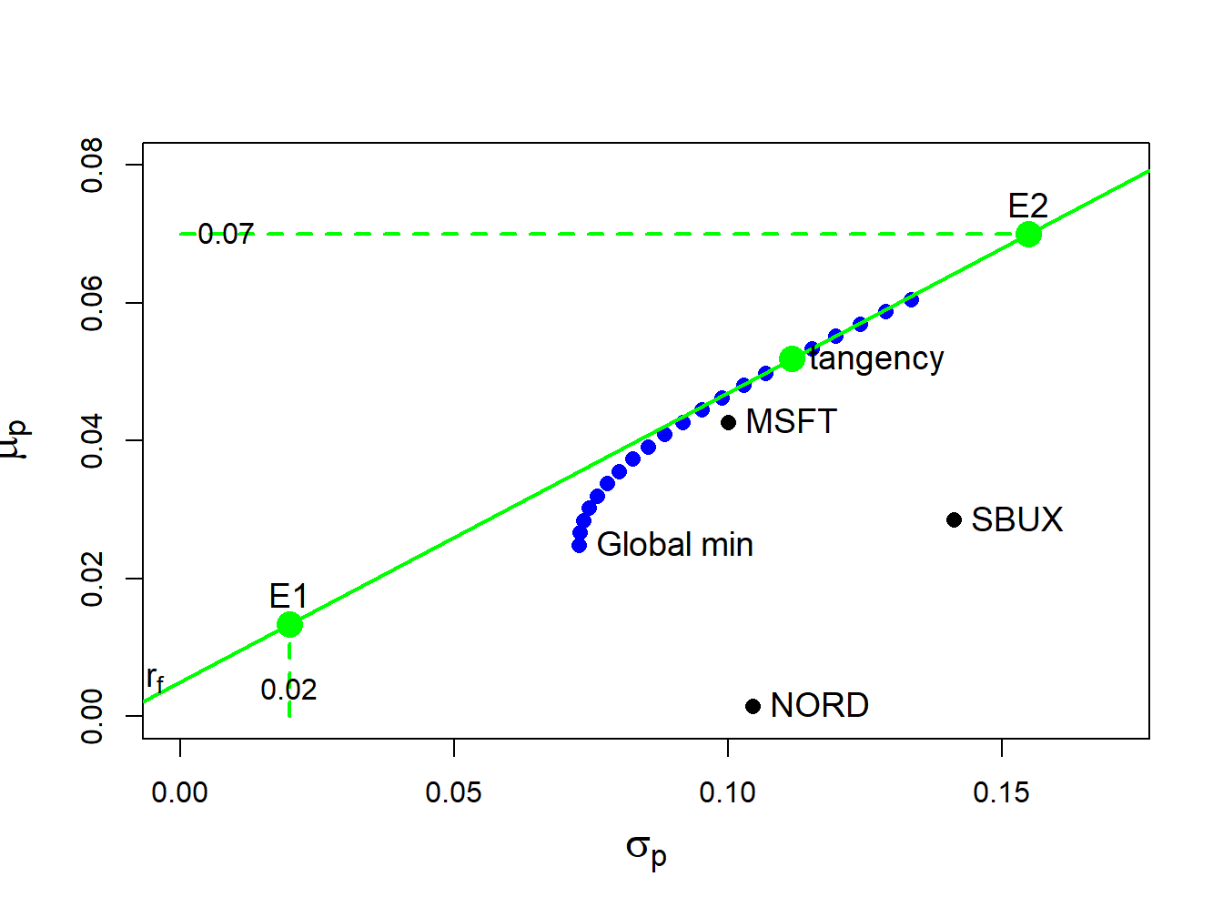
Figure 12.10: Tangency portfolio

For a mathematical proof of these results, see Ingersoll (1987).↩︎