10.1 Engle’s ARCH Model
- Goal: create a simple time series model that captures the basic stylized facts of daily return data
- Foundation of the field of financial econometrics
10.1.1 The ARCH(1) Model
Let \(R_{t}\) denote the continuously compounded daily return on an asset. The CER model for \(R_{t}\) can be expressed in the form: \[\begin{eqnarray} R_{t} & = & \mu+\epsilon_{t},\,t=1,\ldots,T,\tag{10.1}\\ \epsilon_{t} & = & \sigma z_{t},\tag{10.2}\\ z_{t} & \sim & iid\,N(0,1).\tag{10.3} \end{eqnarray}\] Here, the unexpected return \(\epsilon_{t}\) is expressed as \(\sigma z_{t}\) where \(\sigma\) is the unconditional volatility of \(\epsilon_{t}\), which is assumed to be constant, and \(z_{t}=\epsilon_{t}/\sigma\) is the standardized unexpected return. In (10.1)-(10.3), \(R_{t}\sim iid\,N(\mu,\sigma^{2})\) which is not a good model for daily returns given the stylized facts. The ARCH(1) model for \(R_{t}\) has a similar form: \[\begin{eqnarray} R_{t} & = & \mu+\epsilon_{t},\,t=1,\ldots,T,\tag{10.4}\\ \epsilon_{t} & = & \sigma_{t}z_{t},\tag{10.5}\\ \sigma_{t}^{2} & = & \omega+\alpha_{1}\epsilon_{t-1}^{2},\tag{10.6}\\ z_{t} & \sim & iid\,N(0,1),\tag{10.7}\\ \omega>0, & & 0\leq\alpha_{1}<1.\tag{10.8} \end{eqnarray}\]
In the ARCH(1), the unexpected return \(\epsilon_{t}\) is expressed as \(\sigma_{t}z_{t}\) where \(\sigma_{t}\) is the conditional (time \(t\) dependent) volatility of \(\epsilon_{t}\). Hence, the ARCH(1) model extends the CER model to allow for time varying conditional volatility \(\sigma_{t}.\)
In the ARCH(1) model (10.4) - (10.8), the restrictions \(\omega>0\) and \(0\leq\alpha_{1}<1\) are required to ensure that \(\sigma_{t}^{2}>0\) and that \(\{R_{t}\}\) is a covariance stationary time series. Equation (10.6) shows that the return variance at time \(t\), \(\sigma_{t}^{2}\) is a positive linear function of the squared unexpected return at time \(t-1\), \(\epsilon_{t-1}^{2}\). This allows the magnitude of yesterday’s return to influence today’s return variance and volatility. In particular, a large (small) value of \(\epsilon_{t-1}^{2}\) leads to a large (small) value of \(\sigma_{t}^{2}\). This feedback from \(\epsilon_{t-1}^{2}\) to \(\sigma_{t}^{2}\) can explain some of the volatility clustering observed in daily returns.
10.1.1.1 Statistical properties of the ARCH(1) Model
Let \(I_{t}=\{R_{t},R_{t-1},\ldots,R_{1}\}\) denote the information set at time \(t\) (conditioning set of random variables) as described in Chapter 4. As we shall show below, the ARCH(1) model (10.4) - (10.8) has the following statistical properties:
- \(E(\epsilon_{t}|I_{t})=0,\) \(E(\epsilon_{t})=0\).
- \(\mathrm{var}(R_{t}|I_{t})=E(\epsilon_{t}^{2}|I_{t})=\sigma_{t}^{2}\).
- \(\mathrm{var}(R_{t})=E(\epsilon_{t}^{2})=E(\sigma_{t}^{2})=\omega/(1-\alpha_{1})\).
- \(\{R_{t}\}\) is an uncorrelated process: \(\mathrm{cov}(R_{t},R_{t-k})=E(\epsilon_{t}\epsilon_{t-j})=0\) for \(k>0\).
- The distribution of \(R_{t}\) conditional on \(I_{t-1}\) is normal with mean \(\mu\) and variance \(\sigma_{t}^{2}\).
- The unconditional (marginal) distribution of \(R_{t}\) is not normal and \(\mathrm{kurt}(R_{t})\geq3\).
- \(\{R_{t}^{2}\}\) and \(\{\epsilon_{t}^{2}\}\) have a covariance stationary AR(1) model representation. The persistence of the autocorrelations is measured by \(\alpha_{1}.\)
These properties of the ARCH(1) model match many of the stylized facts of daily asset returns.
It is instructive to derive each of the above properties as the derivations make use of certain results and tricks for manipulating conditional expectations. First, consider the derivation for property 1. Because \(\sigma_{t}^{2}=\omega+\alpha_{1}\epsilon_{t-1}^{2}\) depends on information dated \(t-1\), \(\sigma_{t}^{2}\in I_{t-1}\) and so \(\sigma_{t}^{2}\) may be treated as a constant when conditioning on \(I_{t-1}.\) Hence, \[ E(\epsilon_{t}|I_{t})=E(\sigma_{t}z_{t}|I_{t-1})=\sigma_{t}E(z_{t}|I_{t-1})=0. \] The last equality follows from that fact that \(z_{t}\sim iid\,N(0,1)\) which implies that \(z_{t}\) is independent of \(I_{t-1}\) and so \(E(z_{t}|I_{t-1})=E(z_{t})=0\). By iterated expectations, it follows that \[ E(\epsilon_{t})=E(E(\epsilon|I_{t-1}))=E(0)=0. \] The derivation of the second property uses similar computations: \[ \mathrm{var}(R_{t}|I_{t})=E((R_{t}-\mu)^{2}|I_{t-1})=E(\epsilon_{t}^{2}|I_{t})=E(\sigma_{t}^{2}z_{t}^{2}|I_{t-1})=\sigma_{t}^{2}E(z_{t}^{2}|I_{t-1})=\sigma_{t}^{2}, \] where the last equality uses the result \(E(z_{t}^{2}|I_{t-1})=E(z_{t}^{2})=1\).
To derive property 3, first note that by iterated expectations and property 2 \[ \mathrm{var}(R_{t})=E(\epsilon_{t}^{2})=E(E(\epsilon_{t}^{2}|I_{t}))=E(\sigma_{t}^{2}). \]
Next, using (10.6) we have that \[ E(\sigma_{t}^{2})=\omega+\alpha_{1}E(\epsilon_{t-1}^{2}). \] Now use the fact that \(\{R_{t}\}\), and hence \(\{\epsilon_{t}\}\), is covariance stationary which implies that \(E(\epsilon_{t}^{2})=E(\epsilon_{t-1}^{2})=E(\sigma_{t}^{2})\) so that \[ E(\sigma_{t}^{2})=\omega+\alpha_{1}E(\sigma_{t}^{2}). \] Solving for \(E(\sigma_{t}^{2})\) then gives \[ \mathrm{var}(R_{t})=E(\sigma_{t}^{2})=\frac{\omega}{1-\alpha_{1}}. \]
For the fourth property, first note that \[ \mathrm{cov}(R_{t},R_{t-k})=E((R_{t}-\mu)(r_{t-j}-\mu))=E(\epsilon_{t}\epsilon_{t-k})=E(\sigma_{t}z_{t}\sigma_{t-j}z_{t-j}). \] Next, by iterated expectations and the fact that \(z_{t}\sim iid\,N(0,1)\) we have \[ E(\sigma_{t}z_{t}\sigma_{t-j}z_{t-j})=E(E(\sigma_{t}z_{t}\sigma_{t-j}z_{t-j}|I_{t-1}))=E(\sigma_{t}\sigma_{t-j}z_{t-j}E(z_{t}|I_{t-1}))=0, \] and so \(\mathrm{cov}(R_{t},R_{t-k})=0\).
To derive the fifth property, write \(R_{t}=\mu+\epsilon_{t}=\mu+\sigma_{t}z_{t}.\) Then, conditional on \(I_{t-1}\) and the fact that \(z_{t}\sim iid\,N(0,1)\) we have \[ R_{t}|I_{t-1}\sim N(\mu,\sigma_{t}^{2}). \]
The sixth property has two parts. To see that the unconditional distribution of \(R_{t}\) is not a normal distribution, it is useful to express \(R_{t}\) in terms of current and past values of \(z_{t}\) . Start with \[ R_{t}=\mu+\sigma_{t}z_{t}. \] From (10.6), \(\sigma_{t}^{2}=\omega+\alpha_{1}\epsilon_{t-1}^{2}=\omega+\alpha_{1}\sigma_{t-1}^{2}z_{t-1}^{2}\) which implies that \(\sigma_{t}=(\omega+\alpha_{1}\sigma_{t-1}^{2}z_{t-1}^{2})^{1/2}\). Then \[ R_{t}=\mu+(\omega+\alpha_{1}\sigma_{t-1}^{2}z_{t-1}^{2})^{1/2}z_{t}. \]
Even though \(z_{t}\sim iid\,N(0,1)\), \(R_{t}\) is a complicated nonlinear function of \(z_{t}\) and past values of \(z_{t}^{2}\) and so \(R_{t}\) cannot be a normally distributed random variable. Next, to see that \(\mathrm{kurt}(R_{t})\geq3\) first note that \[\begin{equation} \mathrm{kurt}(R_{t})=\frac{E((R_{t}-\mu)^{4})}{\mathrm{var}(R_{t})^{2}}=\frac{E(\epsilon_{t}^{4})}{\omega^{2}/(1-\alpha_{1})^{2}}\tag{10.9} \end{equation}\] Now by iterated expectations and the fact that \(E(z_{t}^{4})=3\) \[ E(\epsilon_{t}^{4})=E(E(\sigma_{t}^{4}z_{t}^{4}|I_{t-1}))=E(\sigma_{t}^{4}E(z_{t}^{4}|I_{t-1}))=3E(\sigma_{t}^{4}). \] Next, using \[\begin{eqnarray*} \sigma_{t}^{4} & = & (\sigma_{t}^{2})^{2}=(\omega+\alpha_{1}\epsilon_{t-1}^{2})^{2}\\ & = & \omega^{2}+2\omega\alpha_{1}\epsilon_{t-1}^{2}+\alpha_{1}^{2}\epsilon_{t-1}^{4} \end{eqnarray*}\] we have \[\begin{eqnarray*} E(\epsilon_{t}^{4}) & = & 3E(\omega^{2}+2\omega\alpha_{1}\epsilon_{t-1}^{2}+\alpha_{1}^{2}\epsilon_{t-1}^{4})\\ & = & 3\omega^{2}+6\omega\alpha_{1}E(\epsilon_{t-1}^{2})+3\alpha_{1}^{2}E(\epsilon_{t-1}^{4}). \end{eqnarray*}\] Since \(\{R_{t}\}\) is covariance stationary it follows that \(E(\epsilon_{t-1}^{2})=E(\epsilon_{t}^{2})=E(\sigma_{t}^{2})=\omega/(1-\alpha_{1})\) and \(E(\epsilon_{t-1}^{4})=E(\epsilon_{t}^{4})\). Hence \[\begin{eqnarray*} E(\epsilon_{t}^{4}) & = & 3\omega^{2}+6\omega\alpha_{1}(\omega/(1-\alpha_{1}))+3\alpha_{1}^{2}E(\epsilon_{t}^{4})\\ & = & 3\omega^{2}\left(1+2\frac{\alpha_{1}}{1-\alpha_{1}}\right)+3\alpha_{1}^{2}E(\epsilon_{t}^{4}). \end{eqnarray*}\] Solving for \(E(\epsilon_{t}^{4})\) gives \[ E(\epsilon_{t}^{4})=\frac{3\omega^{2}(1+\alpha_{1})}{(1-\alpha_{1})(1-3\alpha_{1}^{2})}. \] Because \(0\leq\alpha_{1}<1\), in order for \(E(\epsilon_{t}^{4})<\infty\) it must be the case that \(1-3\alpha_{1}^{2}>0\) which implies that \(0\leq\alpha_{1}^{2}<\frac{1}{3}\) or \(0\leq\alpha_{1}<0.577\). Substituting the above expression for \(E(\epsilon_{t}^{4})\) into (10.9) then gives \[\begin{eqnarray*} \mathrm{kurt}(R_{t}) & = & \frac{3\omega^{2}(1+\alpha_{1})}{(1-\alpha_{1})(1-3\alpha_{1}^{2})}\times\frac{(1-\alpha_{1})^{2}}{\omega^{2}}\\ & = & 3\frac{1-\alpha_{1}^{2}}{1-3\alpha_{1}^{2}}\geq3. \end{eqnarray*}\] Hence, if returns follow an ARCH(1) process with \(\alpha_{1}>0\) then \(\mathrm{kurt}(R_{t})>3\) which implies that the unconditional distribution of returns has fatter tails than the normal distribution.
To show the last property, add \(\epsilon_{t-1}^{2}\) to both sides of (10.6) to give \[\begin{eqnarray*} \epsilon_{t}^{2}+\sigma_{t}^{2} & = & \omega+\alpha_{1}\epsilon_{t-1}^{2}+\epsilon_{t}^{2}\Rightarrow\\ \epsilon_{t}^{2} & = & \omega+\alpha_{1}\epsilon_{t-1}^{2}+\epsilon_{t}^{2}-\sigma_{t}^{2}\\ & = & \omega+\alpha_{1}\epsilon_{t-1}^{2}+v_{t}, \end{eqnarray*}\] where \(v_{t}=\epsilon_{t}^{2}-\sigma_{t}^{2}\) is a mean-zero and uncorrelated error term. Hence, \(\epsilon_{t}^{2}\) and \(R_{t}^{2}\) follow an AR(1) process with positive autoregressive coefficient \(\alpha_{1}.\) The autocorrelations of \(R_{t}^{2}\) are \[ \mathrm{cor}(R_{t}^{2},R_{t-j}^{2})=\alpha_{1}^{j}\,for\,j>1, \] which are positive and decay toward zero exponentially fast as \(j\) gets large. Here, the persistence of the autocorrelations is measured by \(\alpha_{1}.\)
To be completed
\(\blacksquare\)
10.1.1.2 The rugarch package
- Give a brief introduction to the rugarch package
Consider the simple ARCH(1) model for returns \[\begin{align*} R_{t} & =\varepsilon_{t}=\sigma_{t}z_{t},\text{ }z_{t}\sim iid\text{ }N(0,1)\\ \sigma_{t}^{2} & =0.5+0.5R_{t-1}^{2} \end{align*}\] Here, \(\alpha_{1}=0.5<1\) so that \(R_{t}\) is covariance stationary and \(\bar{\sigma}^{2}=\omega/(1-\alpha_{1})=0.5/(1-0.5)=1.\) Using (10.9), \[ \mathrm{kurt}(R_{t})=3\frac{1-\alpha_{1}^{2}}{1-3\alpha_{1}^{2}}=3\frac{1-(0.5)^{2}}{1-3(0.5)^{2}}=9, \] so that the distribution of \(R_{t}\) has much fatter tails than the normal distribution.
The rugarch functions ugarchspec() and ugarchpath()
can be used to simulate \(T=1000\) values of \(R_{t}\) and \(\sigma_{t}\)
from this model.53 The ARCH(1) model is specified using the ugarchpath() function
as follows
## Loading required package: parallel##
## Attaching package: 'rugarch'## The following object is masked from 'package:stats':
##
## sigma## Loading required package: xts## Loading required package: zoo##
## Attaching package: 'zoo'## The following objects are masked from 'package:base':
##
## as.Date, as.Date.numeric##
## Attaching package: 'PerformanceAnalytics'## The following object is masked from 'package:graphics':
##
## legendarch1.spec = ugarchspec(variance.model = list(garchOrder=c(1,0)),
mean.model = list(armaOrder=c(0,0)),
fixed.pars=list(mu = 0, omega=0.5, alpha1=0.5))The argument fixed.pars is a list whose components give the
ARCH(1) model parameters. The names of the list components match the
parameters from the ARCH(1) model: mu is \(\mu\), omega
is \(\omega\), and alpha1 is \(\alpha_{1}.\) Simulated values
of \(R_{t}\) and \(\sigma_{t}\) are produced using the ugarchpath()
function taking as input the "uGARCHspec" object arch1.spec
and the number of simulations, n.sim=1000, to produce:
## [1] "uGARCHpath"
## attr(,"package")
## [1] "rugarch"## [1] "path" "model" "seed"## [1] "sigmaSim" "seriesSim" "residSim"The object arch1.sim is an Sv4 object of class uGARCHpath
for which there are sigma, fitted, quantile,
show and plot methods.54 The path slot is a list which contains the simulated values
of \(\sigma_{t},\) \(R_{t}\) and \(\varepsilon_{t}=R_{t}-\mu_{t}\) as
matrix objects. The method functions sigma() and
fitted() extract \(\sigma_{t}\) and \(\mu_{t},\) respectively.
Invoking the plot() method produces a menu of plot choices
Individual plots can be produced directly by specifying the plot number
in the call to plot(). For example, Figure 10.1
shows the plots of the simulated values for \(R_{t}\) and \(\sigma_{t}\)
created with
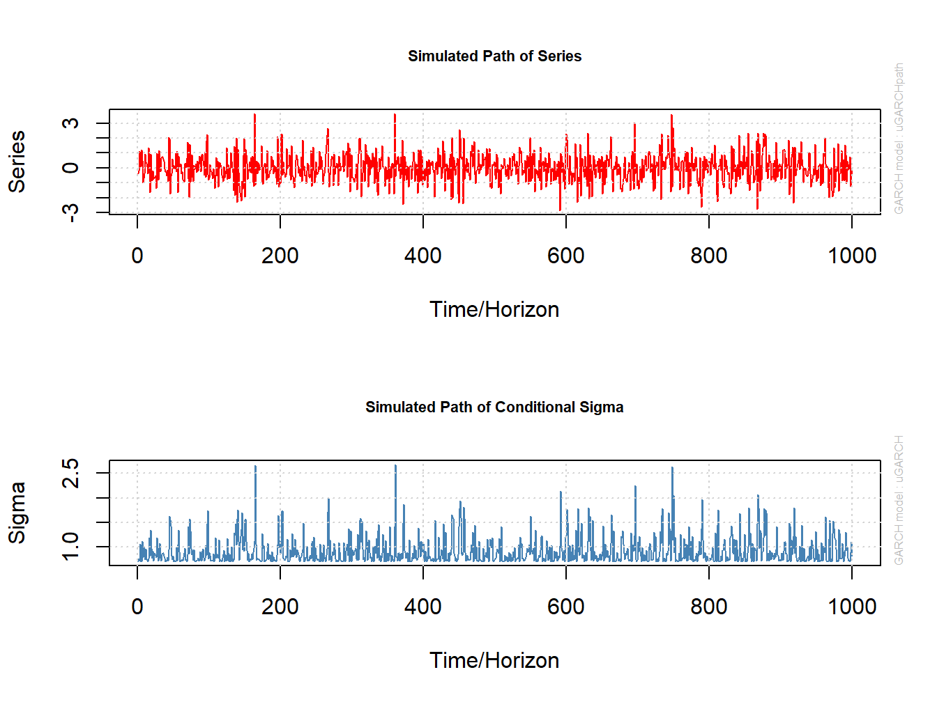
Figure 10.1: Simulated values from ARCH(1) process. Top panel: simulated values of \(R_{t}\). Bottom panel: simulated values of \(\sigma_{t}.\)
Figure 10.2 shows the sample autocorrelations of \(R_{t}\) and \(R_{t}^{2}\). As expected returns are uncorrelated whereas \(R_{t}^{2}\) has autocorrelations described by an AR(1) process with positive autoregressive coefficient\(.\)
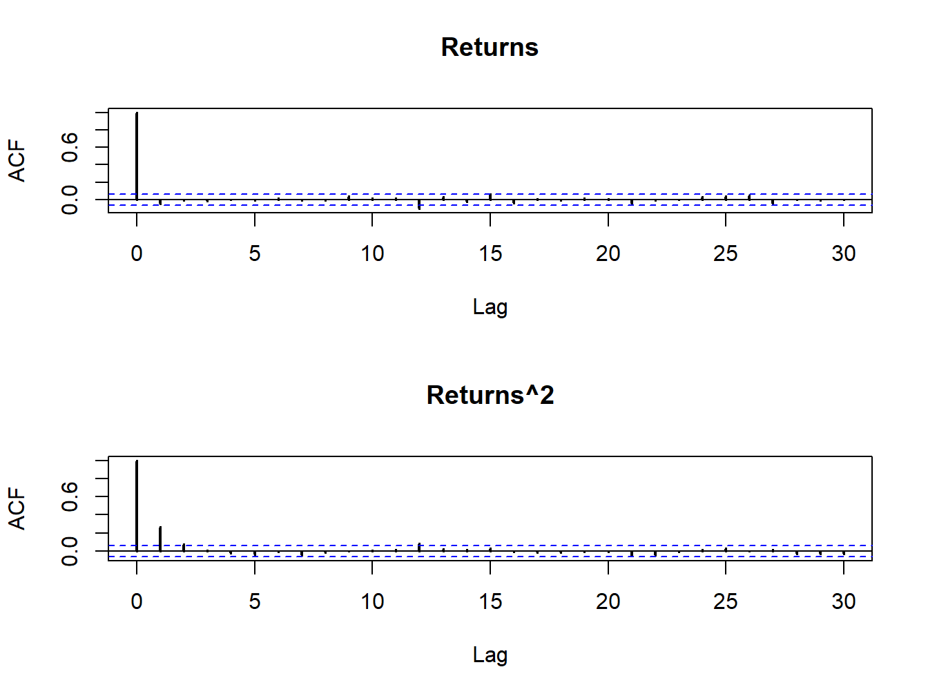
Figure 10.2: SACFs for \(R_{t}\)(top panel) and \(R_{t}^{2}\) (bottom panel) from simulated ARCH(1) model.
The sample variance and excess kurtosis of the simulated returns are
## [1] 0.875674## [1] 0.6495096The sample variance is very close to the unconditional variance \(\bar{\sigma}^{2}=0.2\), and the sample excess kurtosis is very close to the ARCH(1) excess kurtosis of \(6\).
\(\blacksquare\)
10.1.2 The ARCH(p) Model
The ARCH(p) model extends the autocorrelation structure of \(R_{t}^{2}\) and \(\epsilon_{t}^{2}\) in the ARCH(1) model (10.4) - (10.6) to that of an AR(p) process by adding \(p\) lags of \(\epsilon_{t}^{2}\) to the dynamic equation for \(\sigma_{t}^{2}:\) \[\begin{eqnarray} \sigma_{t}^{2} & = & \omega+\alpha_{1}\epsilon_{t-1}^{2}+\alpha_{2}\epsilon_{t-2}^{2}+\cdots+\alpha_{p}\epsilon_{t-p}^{2},\tag{10.10} \end{eqnarray}\] In order for \(\sigma_{t}^{2}\) to be positive we need to impose the restrictions \[\begin{equation} \omega>0,\,\alpha_{1}\geq0,\,\alpha_{2}\geq0,\,\ldots,\alpha_{p}\geq0.\tag{10.11} \end{equation}\] In addition, for \(\{R_{t}\}\) to be a covariance stationary time series we must have the restriction \[\begin{equation} 0\leq\alpha_{1}+\alpha_{2}+\cdots+\alpha_{p}<1.\tag{10.12} \end{equation}\] The statistical properties of the ARCH(p) model are the same as those for the ARCH(1) model with the following exceptions. The unconditional variance of \(\{R_{t}\}\) is \[\begin{equation} \mathrm{var}(R_{t})=E(\epsilon_{t}^{2})=E(\sigma_{t}^{2})=\omega/(1-\alpha_{1}-\alpha_{2}-\cdots-\alpha_{p}),\tag{10.13} \end{equation}\] and \(\{R_{t}^{2}\}\) and \(\{\epsilon_{t}^{2}\}\) have a covariance stationary AR(p) model representation whose autocorrelation persistence is measured by the sum of the ARCH coefficients \(\alpha_{1}+\alpha_{2}+\cdots+\alpha_{p}\).
The ARCH(p) model is capable of creating a much richer autocorrelation structure for \(R_{t}^{2}\). In the ARCH(1) model, the autocorrelations of \(R_{t}^{2}\) decay to zero fairly quickly whereas the sample autocorrelations shown in Figure 10.2 decay to zero very slowly. In the ARCH(p) model, because of the restrictions (10.11) and (10.12), for large values of \(p\) the dynamics of \(\sigma_{t}^{2}\) from (10.10) can more closely mimic the observed autocorrelations of actual daily returns.
To be completed. Simulate long order AR(10) to show difference with ARCH(1). Make sum of ARCH coefficients equal to 0.9
\(\blacksquare\)
More details on using the rugarch functions are given later in the chapter.↩︎
In R there are two main object types: Sv3 and Sv4. The main operational difference between Sv3 and Sv4 objects is that Sv4 components are extracted using the
@character instead of the$character. Also, the names of Sv4 objects are extracted using theslotNames()function instead of thenames()function. ↩︎