13.2 Portfolio Theory with Short Sales Constraints in a Simplified Setting
In this section, we illustrate the impact of short sales constraints on risky assets on portfolios in the simplified setting described in Chapter 11. We first look at simple portfolios of two risky assets, then consider portfolios of a risky asset plus a risk-free asset, and finish with portfolios of two risky assets plus a risk-free asset.
13.2.1 Two Risky Assets
Consider the two risky asset example data from Chapter 11:
mu.A = 0.175
sig.A = 0.258
sig2.A = sig.A^2
mu.B = 0.055
sig.B = 0.115
sig2.B = sig.B^2
rho.AB = -0.164
sig.AB = rho.AB*sig.A*sig.B
assetNames = c("Asset A", "Asset B")
mu.vals = c(mu.A, mu.B)
names(mu.vals) = assetNames
Sigma = matrix(c(sig2.A, sig.AB, sig.AB, sig2.B), 2, 2)
colnames(Sigma) = rownames(Sigma) = assetNames
Asset A is the high average return and high risk asset, and asset B is the low average return and low risk asset. Consider the following set of 19 portfolios:
x.A = seq(from=-0.4, to=1.4, by=0.1)
x.B = 1 - x.A
n.port = length(x.A)
names(x.A) = names(x.B) = paste("p", 1:n.port, sep=".")
mu.p = x.A*mu.A + x.B*mu.B
sig2.p = x.A^2 * sig2.A + x.B^2 * sig2.B + 2*x.A*x.B*sig.AB
sig.p = sqrt(sig2.p)
Figure 13.1 shows the risky asset only portfolio frontier created using:
cex.val = 1.5
plot(sig.p, mu.p, type="b", pch=16, cex = cex.val,
ylim=c(0, max(mu.p)), xlim=c(0, max(sig.p)),
xlab=expression(sigma[p]), ylab=expression(mu[p]), cex.lab=cex.val,
col=c(rep("lightblue", 4), rep("black", 11), rep("lightblue", 4)))
text(x=sig.A, y=mu.A, labels="Asset A", pos=4, cex = cex.val)
text(x=sig.B, y=mu.B, labels="Asset B", pos=4, cex = cex.val)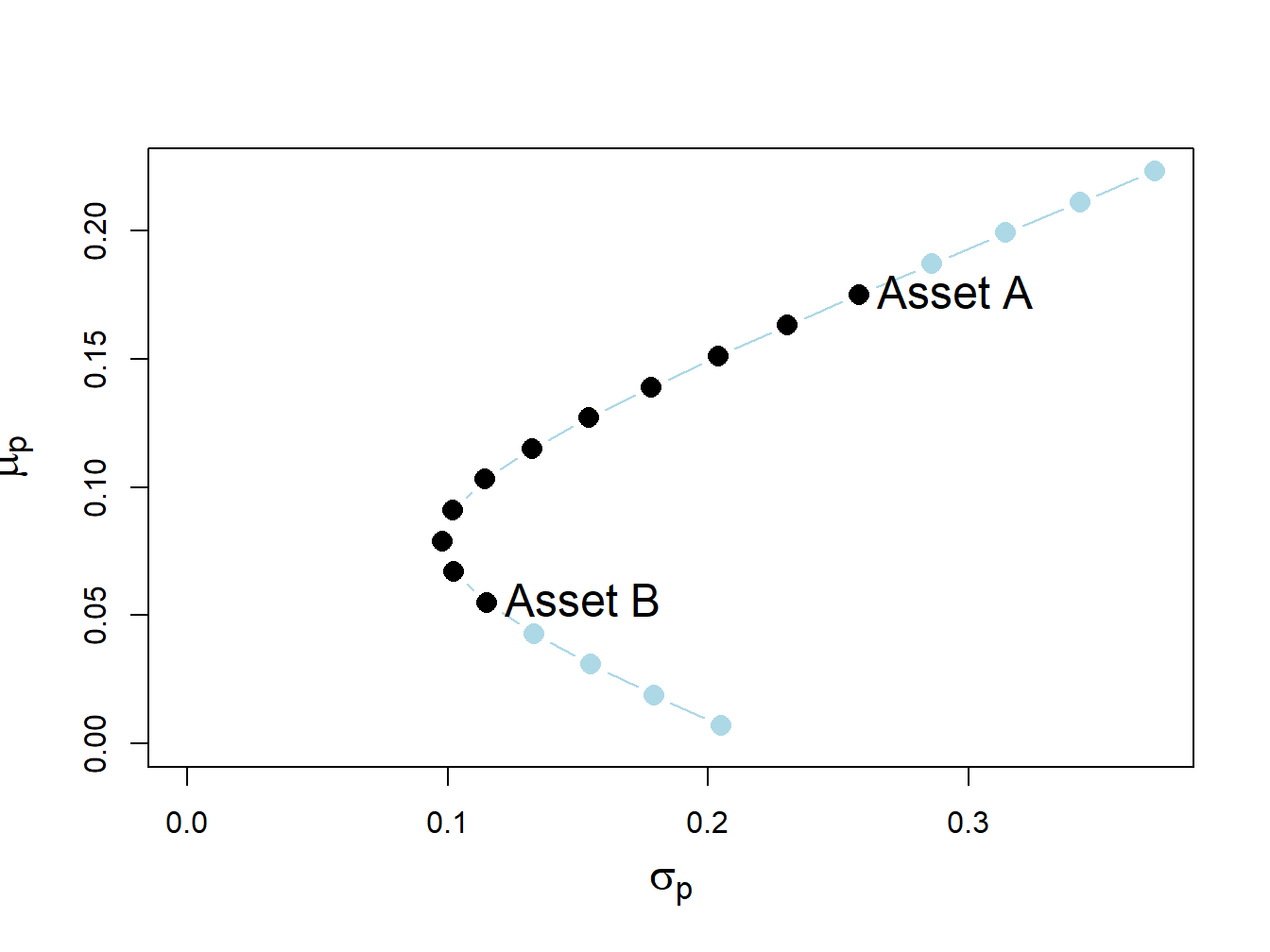
Figure 13.1: Two-risky asset portfolio frontier. Long-only portfolios are in black (between Asset B and Asset A), and long-short portfolios are in blue (below Asset B and above Asset A).
The long only (no short sale) portfolios, shown in black dots between the points labeled “Asset B” and “Asset A”, are portfolios 5 to 15. The asset weights on these portfolios are:
##         p.5 p.6 p.7 p.8 p.9 p.10 p.11 p.12 p.13 p.14 p.15
## Asset A   0 0.1 0.2 0.3 0.4  0.5  0.6  0.7  0.8  0.9    1
## Asset B   1 0.9 0.8 0.7 0.6  0.5  0.4  0.3  0.2  0.1    0
The long-short portfolios, shown in blue dots below the point labeled “Asset B” and above the point labeled “Asset A”, are portfolios 1 to 4 and portfolios 16 to 19:
longShort = rbind(x.A[c(1:4, 16:19)], x.B[c(1:4, 16:19)])
rownames(longShort) = assetNames
longShort
## p.1 p.2 p.3 p.4 p.16 p.17 p.18 p.19
## Asset A -0.4 -0.3 -0.2 -0.1 1.1 1.2 1.3 1.4
## Asset B 1.4 1.3 1.2 1.1 -0.1 -0.2 -0.3 -0.4Not allowing short sales for asset A eliminates the inefficient portfolios 1 to 4 (blue dots below the label “Asset B” ), and not allowing short sales for asset B eliminates the efficient portfolios 16 to 19 (blue dots above the label “Asset A” ). We make the following remarks:
- Not allowing short sales in both assets limits the set of feasible portfolios.
- It is not possible to invest in a portfolio with a higher expected return than asset A.
- It is not possible to invest in a portfolio with a lower expected return than asset B.
13.2.1.1 Short sales constraints and the global minimum variance portfolio
Recall, the two risky asset global minimum variance portfolio solves the unconstrained optimization problem: \[\begin{align*} &\underset{m_{A},m_{B}}{\min}\sigma_{p}^{2} =m_{A}^{2}\sigma_{A}^{2}+m_{B}^{2}\sigma_{B}^{2}+2m_{A}m_{B}\sigma_{AB}\\ &s.t.~m_{A}+m_{B} =1. \end{align*}\]
From Chapter 11, the two risky asset unconstrained global minimum variance portfolio weights are:
\[\begin{equation} m_{A}=\frac{\sigma_{B}^{2}-\sigma_{AB}}{\sigma_{A}^{2}+\sigma_{B}^{2}-2\sigma_{AB}},~m_{B}=1-m_{A}.\tag{13.1} \end{equation}\]
For the example data, the unconstrained global minimum variance portfolio weights are both positive:
## Call:
## globalMin.portfolio(er = mu.vals, cov.mat = Sigma)
##
## Portfolio expected return:     0.0793
## Portfolio standard deviation:  0.0978
## Portfolio weights:
## Asset A Asset B
##   0.202   0.798
This means that if we disallow short-sales in both assets we still get the same global minimum variance portfolio weights. In this case, we say that the no short sales constraints are not binding (have no effect) on the solution for the unconstrained optimization problem (13.1). However, it is possible for one of the weights in the global minimum variance portfolio to be negative if correlation between the returns on assets A and B is sufficiently positive. To see this, the numerator in the formula for the global minimum variance weight for asset A can be re-written as:87
\[ \sigma_{B}^{2}-\sigma_{AB}=\sigma_{B}^{2}-\rho_{AB}\sigma_{A}\sigma_{B}=\sigma_{B}^{2}\left(1-\rho_{AB}\frac{\sigma_{A}}{\sigma_{B}}\right). \]
Hence, the weight in asset A in the global minimum variance portfolio will be negative if:
\[\begin{eqnarray*} 1-\rho_{AB}\frac{\sigma_{A}}{\sigma_{B}} & <0 & \Rightarrow\rho_{AB}>\frac{\sigma_{B}}{\sigma_{A}}. \end{eqnarray*}\]
For the example data, this cut-off value for the correlation is:
## [1] 0.446Figure 13.2 shows the two risky asset portfolio frontier computed with \(\rho_{AB}=0.8\). Here, the global minimum variance portfolio is:
rho.AB = 0.8
sig.AB = rho.AB*sig.A*sig.B
Sigma = matrix(c(sig2.A, sig.AB, sig.AB, sig2.B), 2, 2)
gmin.port = globalMin.portfolio(mu.vals, Sigma)
gmin.port
## Call:
## globalMin.portfolio(er = mu.vals, cov.mat = Sigma)
##
## Portfolio expected return: 0.016
## Portfolio standard deviation: 0.099
## Portfolio weights:
## Asset A Asset B
## -0.325 1.325and contains a negative weight in asset A. This portfolio is shown as the green dot in Figure 13.2, and plots below the point labeled “Asset B” . Here, the no-short sales constraint on asset A is a binding constraint: it is not possible to invest in the global minimum variance portfolio without shorting asset A. Visually, we can see that the feasible long-only portfolio with the smallest variance is 100% invested in asset B. This is the no short sales constrained global minimum variance portfolio. Notice that the variance of this portfolio is larger than the variance of the global minimum variance portfolio. This is the cost, in terms of variance, of imposing the no-short sales constraint.
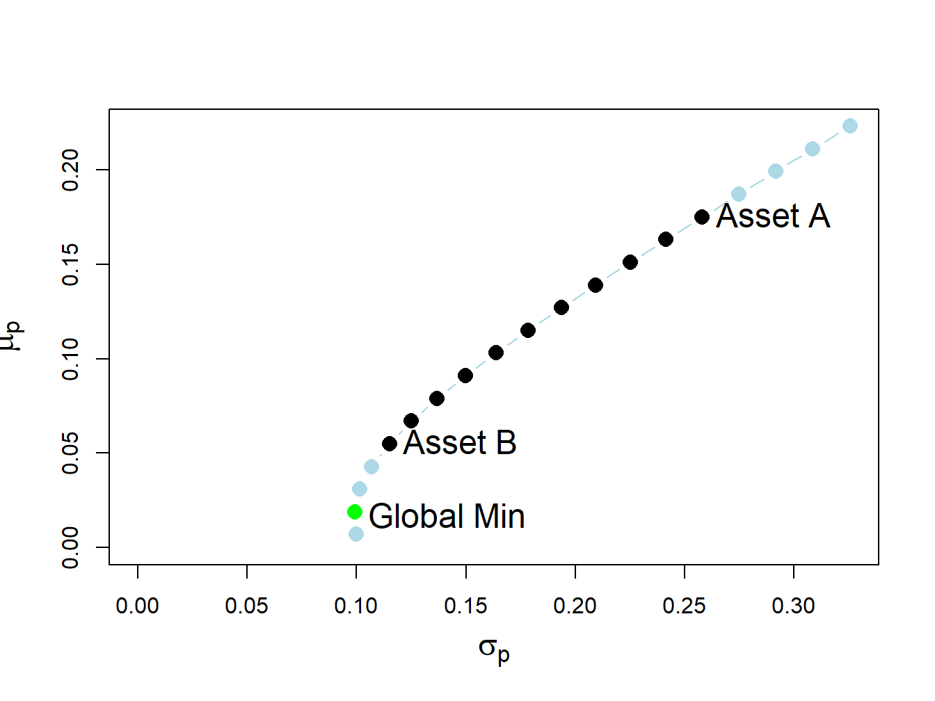
Figure 13.2: Two risky asset portfolio frontier with short sale in Asset A in the global minimum variance portfolio.
13.2.2 One risky asset and a risk-free asset
Now consider portfolios of a risky asset (e.g., asset A) and a risk-free asset (e.g., U.S. T-Bill) with risk-free rate \(r_{f}>0\). Let \(x\) denote the portfolio weight in the risky asset. Then \(1-x\) gives the weight in the risk-free asset. From Chapter 11, the expected return and volatility of portfolios of one risky asset and one risk-free asset are: \[\begin{eqnarray*} \mu_{p} & = & r_{f}+x(\mu-r_{f}),\\ \sigma_{p} & = & |x|\sigma, \end{eqnarray*}\] where \(\mu\) and \(\sigma\) are the expected return and volatility of the risky asset, respectively. For example, Figure 13.3 shows 29 portfolios of asset A and the risk-free asset with \(r_{f}=0.03\) created with:
r.f = 0.03
x.A = seq(from=-1.4, to=1.4, by=0.1)
mu.p.A = r.f + x.A*(mu.A - r.f)
sig.p.A = abs(x.A)*sig.A
plot(sig.p.A, mu.p.A, type="b", ylim=c(min(mu.p.A), max(mu.p.A)),
xlim=c(-0.01, max(sig.p.A)), pch=16, cex = cex.val,
xlab=expression(sigma[p]), ylab=expression(mu[p]), cex.lab = cex.val,
col=c(rep("lightblue", 14), rep("black", 11), rep("lightblue", 4)))
abline(h=0)
text(x=sig.A, y=mu.A, labels="Asset A", pos=4, cex = cex.val)
text(x=0, y=r.f, labels=expression(r[f]), pos=2, cex = cex.val)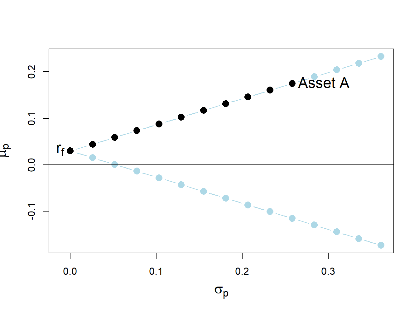
Figure 13.3: Return-risk characteristics of portfolios of asset A and a risk-free asset with \(r_{f}=0.03\). Long-only portfolios are in black (between \(\mathrm{r}_{f}\) and Asset A), and long-short portfolios are in blue (below \(\mathrm{r}_{f}\) and above Asset A).
The portfolios (blue dots) above the point labeled “Asset A” are short the risk-free asset and long more than 100% of asset A. The portfolios (blue dots) below \(r_{f}=0.03\) are short the risky asset and long more than 100% in the risk-free asset.
Here, we assume that the short sales constraint only applies to the risky asset and not the risk-free asset. That is, we assume that we can borrow and lend at the risk-free rate \(r_{f}\) without constraints. In this situation, the no short sales constraint on the risky asset eliminates the inefficient portfolios (blue dots) below the risk-free rate \(r_{f}\).
13.2.3 Two risky assets and risk-free asset
As discussed in Chapter 11, in the case of two risky assets (with no short sales restrictions) plus a risk-free asset the set of efficient portfolios is a combination of the tangency portfolio (i.e., the maximum Sharpe ratio portfolio of two risky assets) and the risk-free asset. For the example data with \(\rho_{AB}=-0.164\) and \(r_{f}=0.03\), the tangency portfolio is:
rho.AB = -0.164
sig.AB = rho.AB*sig.A*sig.B
Sigma = matrix(c(sig2.A, sig.AB, sig.AB, sig2.B), 2, 2)
r.f = 0.03
tan.port = tangency.portfolio(mu.vals, Sigma, r.f)
summary(tan.port, r.f)
## Call:
## tangency.portfolio(er = mu.vals, cov.mat = Sigma, risk.free = r.f)
##
## Portfolio expected return: 0.111
## Portfolio standard deviation: 0.125
## Portfolio Sharpe Ratio: 0.644
## Portfolio weights:
## Asset A Asset B
## 0.463 0.537No asset is sold short in the unconstrained tangency portfolio, and so this is also the short-sales constrained tangency portfolio. The set of efficient portfolios is illustrated in Figure 13.4, created with:
# risky asset only portfolios
x.A = seq(from=0, to=1, by=0.1)
x.B = 1 - x.A
mu.p = x.A*mu.A + x.B*mu.B
sig2.p = x.A^2 * sig2.A + x.B^2 * sig2.B + 2*x.A*x.B*sig.AB
sig.p = sqrt(sig2.p)
# T-bills plus tangency
x.tan = seq(from=0, to=2.4, by=0.1)
mu.p.tan.tbill = r.f + x.tan*(tan.port$er - r.f)
sig.p.tan.tbill = x.tan*tan.port$sd
# global minimum variance portfolio
gmin.port = globalMin.portfolio(mu.vals, Sigma)
# plot efficient portfolios
plot(sig.p, mu.p, type="b", pch=16, cex = cex.val,
     ylim=c(0, 0.20), xlim=c(-0.01, 0.35),
     xlab=expression(sigma[p]), ylab=expression(mu[p]), cex.lab = cex.val)
text(x=sig.A, y=mu.A, labels="Asset A", pos=4, cex = cex.val)
text(x=sig.B, y=mu.B, labels="Asset B", pos=4, cex = cex.val)
text(x=0, y=r.f, labels=expression(r[f]), pos=2, cex = cex.val)
text(x=tan.port$sd, y=tan.port$er, labels="Tangency", pos=2, cex = cex.val)
text(gmin.port$sd, gmin.port$er, labels="Global Min", pos = 4,
     cex = cex.val)
points(sig.p.tan.tbill, mu.p.tan.tbill, type="l", col="green",
       lwd=2, cex = cex.val)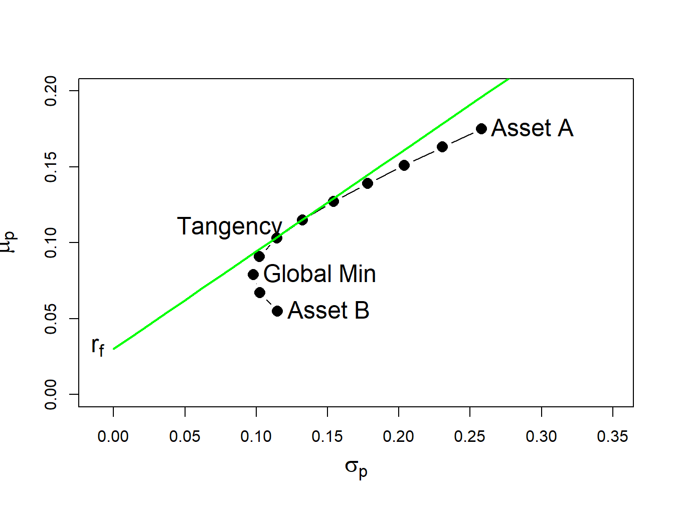
Figure 13.4: Efficient portfolios of two risky assets plus a risk-free asset: \(\rho_{AB}=-0.164\) and \(r_{f}=0.03\). No short sales in unconstrained tangency portfolio.
Figure 13.4 shows that when the tangency portfolio is located between the global minimum variance portfolio (tip of the Markowitz bullet) and asset A, there will be no short sales in the tangency portfolio. However, if the correlation between assets A and B is sufficiently positive (and the risk-free rate is adjusted so that it is greater than the expected return on the global minimum variance portfolio) then asset B can be sold short in the unconstrained tangency portfolio. For example, if \(\rho_{AB}=0.7\) and \(r_{f}=0.01\) the unconstrained tangency portfolio becomes:
rho.AB = 0.7
sig.AB = rho.AB*sig.A*sig.B
Sigma = matrix(c(sig2.A, sig.AB, sig.AB, sig2.B), 2, 2)
r.f = 0.01
tan.port = tangency.portfolio(mu.vals, Sigma, r.f)
summary(tan.port, r.f)
## Call:
## tangency.portfolio(er = mu.vals, cov.mat = Sigma, risk.free = r.f)
##
## Portfolio expected return: 0.238
## Portfolio standard deviation: 0.355
## Portfolio Sharpe Ratio: 0.644
## Portfolio weights:
## Asset A Asset B
## 1.529 -0.529Now, asset B is sold short in the tangency portfolio. The set of efficient portfolios in this case is illustrated in Figure 13.5. Notice that the tangency portfolio is located on the set of risky asset only portfolios above the point labeled “Asset A”, which indicates that asset B is sold short and more than 100% is invested in asset A.88
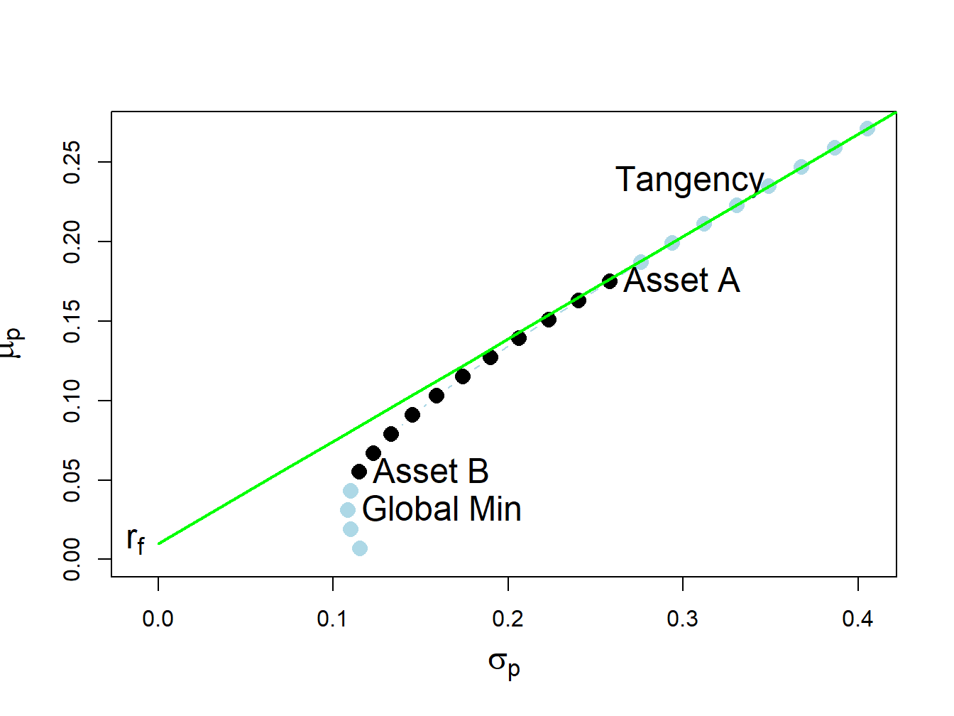
Figure 13.5: Efficient portfolios of two risky assets plus a risk free asset: \(\rho_{AB}=0.7\) and \(r_{f}=0.01\). Asset B sold short in unconstrained tangency portfolio. The short sale constrained tangency portfolio is the point labeled “Asset A”.
When shorts sales of risky assets are not allowed, the unconstrained tangency portfolio is infeasible. In this case, the constrained tangency portfolio is not the tangency portfolio but is 100% invested in asset A. This portfolio is located at the tangency point of a straight line drawn from the risk-free rate to the long-only risky asset frontier. Here, the cost of the no-short sales constraint is the reduction in the Sharpe ratio of the tangency portfolio. The Sharpe ratio of the constrained tangency portfolio is the Sharpe ratio of asset A:
## [1] 0.64Hence, the cost of the no short sales constraint in this example is very small.
By the Cauchy-Schwarz inequality the denominator for \(m_{A}\) in (13.1) is always positive. ↩︎
Also notice that when \(\rho_{AB}=0.7\) the expected return on the global minimum variance drops (frontier of risky assets is shifted down) below \(0.03\) so we need to reduce \(r_{f}\) to \(0.01\) to ensure that the tangency portfolio has a positive slope. ↩︎