12.8 Application to Vanguard Mutual Fund
In this section, we use mean-variance portfolio theory to study asset allocation among a collection of Vanguard mutual Funds. To motivate this example, consider an investor who is deciding how to allocate savings in an employee-sponsored retirement plan.85 Typical plans only allow participants to invest in a limited set of mutual funds. An important limitation of investing in mutual funds is that they cannot be sold short.
The IntroCompFinR data object VanguardPrices contains
monthly closing prices on six diversified and passively managed Vanguard
mutual funds over the period January, 1995 through December, 2014:
## [1] "vfinx" "veurx" "veiex" "vbltx" "vbisx" "vpacx"## [1] "Jan 1995" "Dec 2014"Table 12.3 gives a brief description of the six funds.86
| Fund Ticker | Fund Name | Description |
|---|---|---|
| vfinx | Vanguard 500 Index | Tracks the S&P 500 index |
| veurx | Vanguard European Stock Index | Tracks the MSCI Europe index |
| veiex | Vanguard Emerging Markets Index | Tracks the MSCI Emerging Markets index |
| vbltx | Vanguard Long-Term Bond Index | Tracks a US long-term bond index |
| vbisx | Vanguard Short-Term Bond Index | Tracks a US short-term bond index |
| vpacx | Vanguard Pacific Stock Index | Tracks the MSCI Pacific index |
We construct mean-variance efficient portfolios using annualized GWN model estimates of the expected return vector and covariance matrix based on simple returns over the sub-period January, 2010 through December, 2014. These estimates are computed using:
VanguardRetS = na.omit(Return.calculate(VanguardPrices,
                                        method="simple"))
smpl = "2010-1::2014-12"
muhat = 12*colMeans(VanguardRetS[smpl])
covhat = 12*cov(VanguardRetS[smpl])
The estimated annualized expected returns and standard deviations are:
##  vfinx  veurx  veiex  vbltx  vbisx  vpacx
## 0.1513 0.0723 0.0356 0.0965 0.0196 0.0613## vfinx veurx veiex vbltx vbisx vpacx
## 0.1300 0.1947 0.1914 0.0864 0.0137 0.1467The stock funds have higher average returns and volatilities than the bond funds. The annual risk-free rate at the end of this period is approximately 0.1%. Using this rate, the estimated Sharpe ratios on the six funds are:
## vfinx veurx veiex vbltx vbisx vpacx
## 1.156 0.366 0.181 1.105 1.359 0.411
Interestingly, the short term US bond fund vbisx has the highest estimated annualized Sharpe ratio at 1.36 followed by vfinx (S&P 500 fund) and vbltx (long-term US bond fund). The Sharpe ratios for the other stock funds are much smaller than one.
The estimated return correlation matrix of the six funds is illustrated
in Figure 12.14, created with
the corrplot function corrplot.mixed():
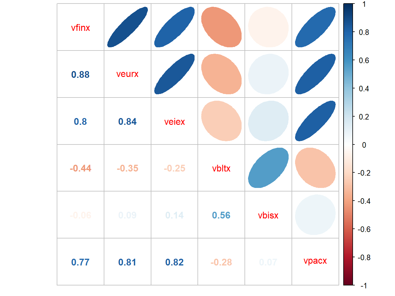
Figure 12.14: Estimated return correlations between six Vanguard mutual funds
The stock funds are all strongly positively correlated with each other, whereas the bond funds are either negatively correlated or very weakly positively correlated with the stock funds. Hence, combining the stock and bond funds in a portfolio should be beneficial in terms of risk diversification.
We use the IntroCompFinR portfolio functions to compute estimates of the global minimum variance portfolio, the tangency portfolio, and the efficient frontier of risky assets:
gmin.port = globalMin.portfolio(muhat, covhat)
tan.port = tangency.portfolio(muhat, covhat, r.f)
ef = efficient.frontier(muhat, covhat, alpha.min=-0.5,
                        alpha.max=1.5, nport=20)
The estimated global minimum variance portfolio is:
## Call:
## globalMin.portfolio(er = muhat, cov.mat = covhat)
##
## Portfolio expected return:     0.0197
## Portfolio standard deviation:  0.0114
## Portfolio weights:
##   vfinx   veurx   veiex   vbltx   vbisx   vpacx
##  0.0581 -0.0347 -0.0214 -0.0736  1.0647  0.0069
This portfolio is mostly concentrated in the short-term US bond fund vbisx (which has the smallest volatility) and has small short positions in veurx, veiex and vbltx. This portfolio is not feasible, however, because investors are not allowed to short sell mutual funds.
The estimated tangency portfolio is:
## Call:
## tangency.portfolio(er = muhat, cov.mat = covhat, risk.free = r.f)
##
## Portfolio expected return:     0.0642
## Portfolio standard deviation:  0.0209
## Portfolio weights:
##   vfinx   veurx   veiex   vbltx   vbisx   vpacx
##  0.3152 -0.0907 -0.0874  0.1159  0.7387  0.0083
This portfolio is also an infeasible long-short portfolio with long positions in the US funds vfinx, vbltx and vbisx and short positions in the non-US stock funds veurx, veiex and vpacx.
The mean-variance efficient frontiers are illustrated in Figure 12.15, created using:
plot(ef, plot.assets=TRUE, col="blue", pch=16)
text(gmin.port$sd, gmin.port$er,labels = "gmin", pos = 2)
text(tan.port$sd, tan.port$er,labels = "tan", pos = 3)
sr.tan = (tan.port$er - r.f)/tan.port$sd
text(0, r.f, labels=expression(r[f]), pos = 4)
abline(a=r.f, b=sr.tan, col="green", lwd=2)
abline(h=0, v=0)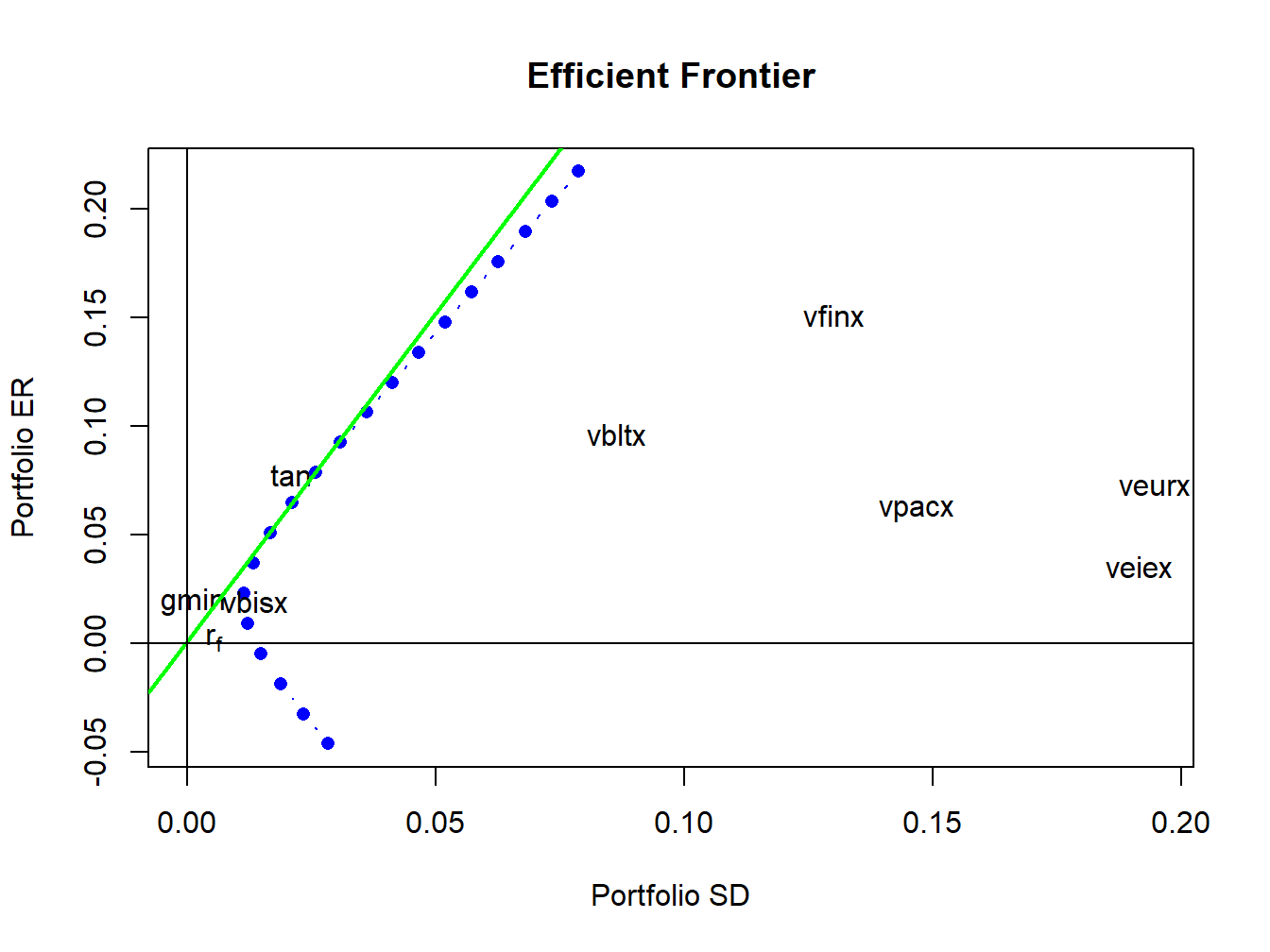
Figure 12.15: Mean variance efficient portfolios of the Vanguard mutual funds. The risky asset portfolio frontier is shown in blue. The efficient portfolios of the risk-free asset and the risky assets is shown in green. The global minimum variance portfolio is labeled “gmin”, and the tangency portfolio is labeled “tan”.
The portfolio frontier of risky assets is shown in blue. These portfolios are infeasible because they all contain short sales in one or more of the mutual funds:
##            vfinx    veurx    veiex     vbltx   vbisx   vpacx
## port 1  -0.32213  0.04799  0.07623 -0.353776  1.5469 0.00480
## port 2  -0.24208  0.03057  0.05568 -0.294783  1.4454 0.00524
## port 3  -0.16203  0.01316  0.03512 -0.235789  1.3439 0.00568
## port 4  -0.08198 -0.00426  0.01456 -0.176795  1.2423 0.00612
## port 5  -0.00193 -0.02167 -0.00599 -0.117802  1.1408 0.00656
## port 6   0.07813 -0.03909 -0.02655 -0.058808  1.0393 0.00700
## port 7   0.15818 -0.05650 -0.04711  0.000186  0.9378 0.00744
## port 8   0.23823 -0.07392 -0.06766  0.059179  0.8363 0.00788
## port 9   0.31828 -0.09133 -0.08822  0.118173  0.7348 0.00832
## port 10  0.39833 -0.10875 -0.10878  0.177167  0.6333 0.00876
## port 11  0.47839 -0.12616 -0.12933  0.236160  0.5318 0.00920
## port 12  0.55844 -0.14358 -0.14989  0.295154  0.4302 0.00964
## port 13  0.63849 -0.16099 -0.17045  0.354148  0.3287 0.01008
## port 14  0.71854 -0.17840 -0.19101  0.413141  0.2272 0.01052
## port 15  0.79859 -0.19582 -0.21156  0.472135  0.1257 0.01096
## port 16  0.87865 -0.21323 -0.23212  0.531128  0.0242 0.01140
## port 17  0.95870 -0.23065 -0.25268  0.590122 -0.0773 0.01183
## port 18  1.03875 -0.24806 -0.27323  0.649116 -0.1788 0.01227
## port 19  1.11880 -0.26548 -0.29379  0.708109 -0.2804 0.01271
## port 20  1.19885 -0.28289 -0.31435  0.767103 -0.3819 0.01315
The locations of vbisx and the global minimum variance portfolio are almost identical, which suggests that vbisx is a good feasible substitute for the infeasible global minimum variance portfolio. The remaining funds are well inside the risky asset efficient frontier. The set of efficient portfolios of risky assets plus the risk-free asset is shown in green. These are portfolios of the risk-free asset and the tangency portfolio. Since the tangency portfolio contains short sales, these portfolios are not feasible. However, the tangency portfolio is approximately 70% vbisx and 30% vfinx so a close substitute for the efficient portfolios are combinations of the risk-free asset and the approximate tangency portfolio that is 70% vbisx and 30% vfinx.
This example highlights some practical problems associated with applying mean-variance portfolio theory in a real-world asset allocation context. In particular, mean-variance efficient portfolios often contain short sales in some assets. When the underlying assets are mutual funds, investors are not allowed to directly short these assets and it may not be possible to exactly implement the theory. The next chapter shows how mean-variance portfolio theory can be modified to allow for additional constraints created by short sales restrictions.