7.5 Statistical Properties of the GWN Model Estimates
To determine the statistical properties of plug-in principle estimators \(\hat{\mu}_{i},\hat{\sigma}_{i}^{2},\hat{\sigma}_{i},\hat{\sigma}_{ij}\) and \(\hat{\rho}_{ij}\) in the GWN model, we treat them as functions of the random variables \(\{\mathbf{R}_{t}\}_{t=1}^{T}\) where \(\mathbf{R}_{t}\) is assumed to be generated by the GWN model (7.1).
7.5.1 Bias
Proposition 7.4 (Bias of GWN model estimators) Assume that returns are generated by the GWN model (7.1). Then the estimators \(\hat{\mu}_{i},\) \(\hat{\sigma}_{i}^{2}\) and \(\hat{\sigma}_{ij}\) are unbiased estimators:36 \[\begin{align*} E[\hat{\mu}_{i}] & =\mu_{i}\\ E[\hat{\sigma}_{i}^{2}] & =\sigma_{i}^{2},\\ E[\hat{\sigma}_{ij}] & =\sigma_{ij}. \end{align*}\] The estimators \(\hat{\sigma}_{i}\) and \(\hat{\rho}_{ij}\) are biased estimators: \[\begin{align*} E[\hat{\sigma}_{i}] & \neq\sigma_{i},\\ E[\hat{\rho}_{ij}] & \neq\rho_{ij}. \end{align*}\]
It can be shown that the biases in \(\hat{\sigma}_{i}\) and \(\hat{\rho}_{ij}\), are very small and decreasing in \(T\) such that \(\mathrm{bias}(\hat{\sigma}_{i},\sigma_{i})=\mathrm{bias}(\hat{\rho}_{ij},\rho_{ij})=0\) as \(T\rightarrow\infty\). The proofs of these results are beyond the scope of this book and may be found, for example, in Goldberger (1991). As we shall see, these results about bias can be easily verified using Monte Carlo methods.
It is instructive to illustrate how to derive the result \(E[\hat{\mu}_{i}]=\mu_{i}\). Using \(\hat{\mu}_{i} = \frac{1}{T}\sum_{t=1}^{T}R_{it}\) and results about the expectation of a linear combination of random variables, it follows that: \[\begin{align*} E[\hat{\mu}_{i}] & =E\left[\frac{1}{T}\sum_{t=1}^{T}R_{it}\right]\\ & =\frac{1}{T}\sum_{t=1}^{T} E[R_{it}]~ (\textrm{by the linearity of }E[\cdot])\\ & =\frac{1}{T}\sum_{t=1}^{T}\mu_{i}~ (\textrm{since }E[R_{it}]=\mu_{i},~t=1,\ldots,T)\\ & =\frac{1}{T}T\cdot\mu_{i}=\mu_{i}. \end{align*}\] The derivation of the results \(E[\hat{\sigma}_{i}^{2}]=\sigma_{i}^{2}\) and \(E[\hat{\sigma}_{ij}]=\sigma_{ij}\) are similar but are considerably more involved and so are omitted.
7.5.2 Precision
Because the GWN model estimators are either unbiased or the bias is very small, the precision of these estimators is measured by their standard errors. Here, we give the mathematical formulas for their standard errors.
Proposition 7.5 (Standard error for \(\hat{\mu_i}\)) The standard error for \(\hat{\mu}_{i},\) \(\mathrm{se}(\hat{\mu}_{i}),\) can be calculated exactly and is given by: \[\begin{equation} \mathrm{se}(\hat{\mu}_{i})=\frac{\sigma_{i}}{\sqrt{T}}.\tag{7.19} \end{equation}\]
The derivation of this result is straightforward. Using the results for the variance of a linear combination of uncorrelated random variables, we have: \[\begin{align*} \mathrm{var}(\hat{\mu}_{i}) & =\mathrm{var}\left(\frac{1}{T}\sum_{t=1}^{T}R_{it}\right)\\ & =\frac{1}{T^{2}}\sum_{t=1}^{T}\mathrm{var}(R_{it})~ (\textrm{since }R_{it}\textrm{ is independent over time})\\ & =\frac{1}{T^{2}}\sum_{t=1}^{T}\sigma_{i}^{2}~ (\textrm{since }\mathrm{var}(R_{it})=\sigma_{i}^{2},~t=1,\ldots,T)\\ & =\frac{1}{T^{2}}T\sigma_{i}^{2}\\ & =\frac{\sigma_{i}^{2}}{T}. \end{align*}\]
Then \(\mathrm{se}(\hat{\mu}_{i})=\mathrm{sd}(\hat{\mu}_{i})=\frac{\sigma_{i}}{\sqrt{T}}\). We make the following remarks:
- The value of \(\mathrm{se}(\hat{\mu}_{i})\) is in the same units as \(\hat{\mu}_{i}\) and measures the precision of \(\hat{\mu}_{i}\) as an estimate. If \(\mathrm{se}(\hat{\mu}_{i})\) is small relative to \(\hat{\mu}_{i}\) then \(\hat{\mu}_{i}\) is a relatively precise estimate of \(\mu_{i}\) because \(f(\hat{\mu}_{i})\) will be tightly concentrated around \(\mu_{i}\); if \(\mathrm{se}(\hat{\mu}_{i})\) is large relative to \(\mu_{i}\) then \(\hat{\mu}_{i}\) is a relatively imprecise estimate of \(\mu_{i}\) because \(f(\hat{\mu}_{i})\) will be spread out about \(\mu_{i}\).
- The magnitude of \(\mathrm{se}(\hat{\mu}_{i})\) depends positively on the volatility of returns, \(\sigma_{i}=\mathrm{sd}(R_{it})\). For a given sample size \(T\), assets with higher return volatility have larger values of \(\mathrm{se}(\hat{\mu}_{i})\) than assets with lower return volatility. In other words, estimates of expected return for high volatility assets are less precise than estimates of expected returns for low volatility assets.
- For a given return volatility \(\sigma_{i}\), \(\mathrm{se}(\hat{\mu}_{i})\) is smaller for larger sample sizes \(T\). In other words, \(\hat{\mu}_{i}\) is more precisely estimated for larger samples.
- \(\mathrm{se}(\hat{\mu}_{i})\rightarrow0\) as \(T\rightarrow\infty\). This together with \(E[\hat{\mu_{i}}]=\mu_{i}\) shows that \(\hat{\mu_{i}}\) is consistent for \(\mu_{i}\).
The derivations of the standard errors for \(\hat{\sigma}_{i}^{2},\hat{\sigma}_{i}\), \(\hat{\sigma}_{ij}\) and \(\hat{\rho}_{ij}\) are complicated, and the exact results are extremely messy and hard to work with. However, there are simple approximate formulas for the standard errors of \(\hat{\sigma}_{i}^{2},\hat{\sigma}_{i}\), \(\hat{\sigma_{ij}}\), and \(\hat{\rho}_{ij}\) based on the CLT under the GWN model that are valid if the sample size, \(T\), is reasonably large.
Proposition 7.6 (Approximate standard error formulas for \(\hat{\sigma}_{i}^{2},\hat{\sigma}_{i}\), \(\hat{\sigma_{ij}}\), and \(\hat{\rho}_{ij}\)) The approximate standard error formulas for \(\hat{\sigma}_{i}^{2},\hat{\sigma}_{i}\), \(\hat{\sigma_{ij}}\), and \(\hat{\rho}_{ij}\) are given by:
\[\begin{align} \mathrm{se}(\hat{\sigma}_{i}^{2}) & \approx\frac{\sqrt{2}\sigma_{i}^{2}}{\sqrt{T}}=\frac{\sigma_{i}^{2}}{\sqrt{T/2}},\tag{7.20}\\ \mathrm{se}(\hat{\sigma}_{i}) & \approx\frac{\sigma_{i}}{\sqrt{2T}},\tag{7.21}\\ \mathrm{se}(\hat{\sigma}_{ij}) & \approx \frac{\sqrt{\sigma_i^2 \sigma_j^2 + \sigma_{ij}^2}}{\sqrt{T}} = \frac{\sqrt{\sigma_i^2 \sigma_j^2 (1 + \rho_{ij}^2)}}{\sqrt{T}} \tag{7.22}\\ \mathrm{se}(\hat{\rho}_{ij}) & \approx\frac{1-\rho_{ij}^{2}}{\sqrt{T}},\tag{7.23} \end{align}\] where “\(\approx\)” denotes approximately equal. The approximations are such that the approximation error goes to zero as the sample size \(T\) gets very large.
We make the following remarks:
- As with the formula for the standard error of the sample mean, the formulas for \(\mathrm{se}(\hat{\sigma}_{i}^{2})\) and \(\mathrm{se}(\hat{\sigma}_{i})\) depend on \(\sigma_{i}^{2}\). Larger values of \(\sigma_{i}^{2}\) imply less precise estimates of \(\hat{\sigma}_{i}^{2}\) and \(\hat{\sigma}_{i}\).
- The formula for \(\mathrm{se}(\hat{\sigma}_{ij})\) depends on \(\sigma_i^2\), \(\sigma_j^2\), and \(\rho_{ij}^2\). Given \(\sigma_i^2\) and \(\sigma_j^2\), the standard error is smallest when \(\rho_{ij}=0\).
- The formula for \(\mathrm{se}(\hat{\rho}_{ij})\), does not depend on \(\sigma_{i}^{2}\) but rather depends on \(\rho_{ij}^{2}\) and is smaller the closer \(\rho_{ij}^{2}\) is to unity. Intuitively, this makes sense because as \(\rho_{ij}^{2}\) approaches one the linear dependence between \(R_{it}\) and \(R_{jt}\) becomes almost perfect and this will be easily recognizable in the data (scatterplot will almost follow a straight line).
- The formulas for the standard errors above are inversely related to the square root of the sample size, \(\sqrt{T}\), which means that larger sample sizes imply smaller values of the standard errors.
- Interestingly, \(\mathrm{se}(\hat{\sigma}_{i})\) goes to zero the fastest and \(\mathrm{se}(\hat{\sigma}_{i}^{2})\) goes to zero the slowest. Hence, for a fixed sample size, these formulas suggest that \(\sigma_{i}\) is generally estimated more precisely than \(\sigma_{i}^{2}\) and \(\rho_{ij}\), and \(\rho_{ij}\) is estimated generally more precisely than \(\sigma_{i}^{2}\).
The above formulas (7.20) - (7.23) are not practically useful, however, because they depend on the unknown quantities \(\sigma_{i}^{2},\sigma_{i}\) and \(\rho_{ij}\). Practically useful formulas make use of the plug-in principle and replace \(\sigma_{i}^{2},\sigma_{i}\) and \(\rho_{ij}\) by the estimates \(\hat{\sigma}_{i}^{2},\hat{\sigma}_{i}\) and \(\hat{\rho}_{ij}\) and give rise to the estimated standard errors: \[\begin{align} \widehat{\mathrm{se}}(\hat{\mu}_{i}) & =\frac{\widehat{\sigma}_{i}}{\sqrt{T}}\tag{7.24}\\ \widehat{\mathrm{se}}(\hat{\sigma}_{i}^{2}) & \approx\frac{\hat{\sigma}_{i}^{2}}{\sqrt{T/2}},\tag{7.25}\\ \widehat{\mathrm{se}}(\hat{\sigma}_{i}) & \approx\frac{\hat{\sigma}_{i}}{\sqrt{2T}},\tag{7.26}\\ \widehat{\mathrm{se}}(\hat{\sigma}_{ij}) & \approx \frac{\sqrt{\hat{\sigma}_i^2 \hat{\sigma}_j^2 (1 + \hat{\rho}_{ij}^2)}}{\sqrt{T}} \tag{7.27}\\ \widehat{\mathrm{se}}(\hat{\rho}_{ij}) & \approx\frac{1-\hat{\rho}_{ij}^{2}}{\sqrt{T}}.\tag{7.28} \end{align}\]
It is good practice to report estimates together with their estimated standard errors. In this way the precision of the estimates is transparent to the user. Typically, estimates are reported in a table with the estimates in one column and the estimated standard errors in an adjacent column.
For Microsoft, Starbucks and S&P 500, the values of \(\widehat{\mathrm{se}}(\hat{\mu}_{i})\) are easily computed in R using:
The values of \(\hat{\mu}_{i}\) and \(\widehat{\mathrm{se}}(\hat{\mu}_{i})\) shown together are:
##         muhat seMuhat
## MSFT  0.00413 0.00764
## SBUX  0.01466 0.00851
## SP500 0.00169 0.00370
For Microsoft and Starbucks, the values of \(\widehat{\mathrm{se}}(\hat{\mu}_{i})\) are similar because the values of \(\hat{\sigma}_{i}\) are similar, and \(\widehat{\mathrm{se}}(\hat{\mu}_{i})\) is smallest for the S&P 500 index. This occurs because \(\hat{\sigma}_{\textrm{sp500}}\) is much smaller than \(\hat{\sigma}_{\textrm{msft}}\) and \(\hat{\sigma}_{\textrm{sbux}}\). Hence, \(\hat{\mu}_{i}\) is estimated more precisely for the S&P 500 index (a highly diversified portfolio) than it is for Microsoft and Starbucks stock (individual assets).
It is tempting to compare the magnitude of \(\hat{\mu}_{i}\) to \(\widehat{\mathrm{se}}(\hat{\mu}_{i})\) to evaluate if \(\hat{\mu}_{i}\) is a precise estimate. A common way to do this is to compute the so-called t-ratio:
##  MSFT  SBUX SP500
## 0.540 1.722 0.457
The t-ratio shows the number of \(\widehat{\mathrm{se}}(\hat{\mu}_{i})\) values \(\hat{\mu}_{i}\) is from zero. For example, \(\hat{\mu}_{msft} = 0.004\) is 0.54 values of \(\widehat{\mathrm{se}}(\hat{\mu}_{msft}) = 0.008\) above zero. This is not very far from zero. In contrast, \(\hat{\mu}_{sbux} = 0.015\) is 1.72 values of \(\widehat{\mathrm{se}}(\hat{\mu}_{sbux}) = 0.008\) above zero. This is moderately far from zero. Because, \(\hat{\mu_{i}}\) represents an average rate of return on an asset it informative to know how far above zero it is likely to be. The farther \(\hat{\mu_{i}}\) is from zero, in units of \(\widehat{\mathrm{se}}(\hat{\mu}_{i})\), the more we are sure that the asset has a positive average rate of return.
\(\blacksquare\)
For Microsoft, Starbucks and S&P 500, the values of \(\widehat{\mathrm{se}}(\hat{\sigma}_{i}^{2})\) and \(\widehat{\mathrm{se}}(\hat{\sigma}_{i})\) (together with the estimates \(\hat{\sigma}_{i}^{2}\) and \(\hat{\sigma}_{i}\) are:
seSigma2hat = sigma2hat/sqrt(n.obs/2)
seSigmahat = sigmahat/sqrt(2*n.obs)
cbind(sigma2hat, seSigma2hat, sigmahat, seSigmahat)
## sigma2hat seSigma2hat sigmahat seSigmahat
## MSFT 0.01004 0.001083 0.1002 0.00540
## SBUX 0.01246 0.001344 0.1116 0.00602
## SP500 0.00235 0.000253 0.0485 0.00261Notice that \(\sigma^{2}\) and \(\sigma\) for the S&P 500 index are estimated much more precisely than the values for Microsoft and Starbucks. Also notice that \(\sigma_{i}\) is estimated more precisely than \(\mu_{i}\) for all assets: the values of \(\widehat{\mathrm{se}}\)(\(\hat{\sigma}_{i})\) relative to \(\hat{\sigma}_{i}\) are much smaller than the values of \(\widehat{\mathrm{se}}\)(\(\hat{\mu}_{i})\) to \(\hat{\mu}_{i}\).
The values of \(\widehat{\mathrm{se}}(\hat{\sigma}_{ij})\) and \(\widehat{\mathrm{se}}(\hat{\rho}_{ij})\) (together with the values of \(\sigma_{ij}\) and \(\hat{\rho}_{ij})\) are:
seCovhat = sqrt(sigma2hat[c("MSFT","MSFT","SBUX")]*sigma2hat[c("SBUX","SP500","SP500")]*(1 + rhohat^2))/sqrt(n.obs)
seRhohat = (1-rhohat^2)/sqrt(n.obs)
cbind(covhat, seCovhat, rhohat, seRhohat)
## covhat seCovhat rhohat seRhohat
## msft,sbux 0.00381 0.000901 0.341 0.0674
## msft,sp500 0.00300 0.000435 0.617 0.0472
## sbux,sp500 0.00248 0.000454 0.457 0.0603The values of \(\widehat{\mathrm{se}}(\hat{\sigma}_{ij})\) and \(\widehat{\mathrm{se}}(\hat{\rho}_{ij})\) are moderate in size (relative to \(\hat{\sigma}_{ij}\) and \(\hat{\rho}_{ij})\). Notice that \(\hat{\rho}_{\textrm{sbux,sp500}}\) has the smallest estimated standard error because \(\hat{\rho}_{\textrm{sbux,sp500}}^{2}\) is closest to one.
\(\blacksquare\)
7.5.3 Sampling Distributions and Confidence Intervals
7.5.3.1 Sampling Distribution for \(\hat{\mu}_{i}\)
In the GWN model, \(R_{it}\sim iid~N(\mu_{i},\sigma_{i}^{2})\) and since \(\hat{\mu}_{i}=\frac{1}{T}\sum_{t=1}^{T}R_{it}\) is an average of these normal random variables, it is also normally distributed. Previously we showed that \(E[\hat{\mu}_{i}]=\mu_{i}\) and \(\mathrm{var}(\hat{\mu}_{i}) =\frac{\sigma_{i}^{2}}{T}\). Therefore, the exact probability distribution of \(\hat{\mu}_{i}\), \(f(\hat{\mu}_{i})\), for a fixed sample size \(T\) is the normal distribution \(\hat{\mu}_{i}\sim~N\left(\mu_{i},\frac{\sigma_{i}^{2}}{T}\right).\) Therefore, we have an exact formula for \(f(\hat{\mu}_{i})\):
\[\begin{equation} f(\hat{\mu}_{i})=\left(\frac{2\pi\sigma_{i}^{2}}{T}\right)^{-1/2}\exp\left\{ -\frac{1}{2\sigma_{i}^{2}/T}(\hat{\mu}_{i}-\mu_{i})^{2}\right\} .\tag{7.29} \end{equation}\]
The probability curve \(f(\hat{\mu}_{i})\) is centered at the true value \(\mu_{i}\), and the spread about \(\mu_{i}\) depends on the magnitude of \(\sigma_{i}^{2}\), the variability of \(R_{it}\), and the sample size, \(T\). For a fixed sample size \(T\), the uncertainty in \(\hat{\mu}_{i}\) is larger (smaller) for larger (smaller) values of \(\sigma_{i}^{2}\). Notice that the variance of \(\hat{\mu}_{i}\) is inversely related to the sample size \(T\). Given \(\sigma_{i}^{2}\), \(\mathrm{var}(\hat{\mu}_{i})\) is smaller for larger sample sizes than for smaller sample sizes. This makes sense since we expect to have a more precise estimator when we have more data. If the sample size is very large (as \(T\rightarrow\infty\)) then \(\mathrm{var}(\hat{\mu}_{i})\) will be approximately zero and the normal distribution of \(\hat{\mu}_{i}\) given by (7.29) will be essentially a spike at \(\mu_{i}\). In other words, if the sample size is very large then we essentially know the true value of \(\mu_{i}\). Hence, we have established that \(\hat{\mu}_{i}\) is a consistent estimator of \(\mu_{i}\) as the sample size goes to infinity.
The exact sampling distribution for \(\hat{\mu}\) assumes that \(\sigma^2\) is known, which is not practically useful. Below, we provide a practically useful result which holds when we use \(\hat{\sigma}^2\).
The distribution of \(\hat{\mu}_{i}\), with \(\mu_{i}=0\) and \(\sigma_{i}^{2}=1\) for various sample sizes is illustrated in figure 7.4. Notice how fast the distribution collapses at \(\mu_{i}=0\) as \(T\) increases.
\(\blacksquare\)
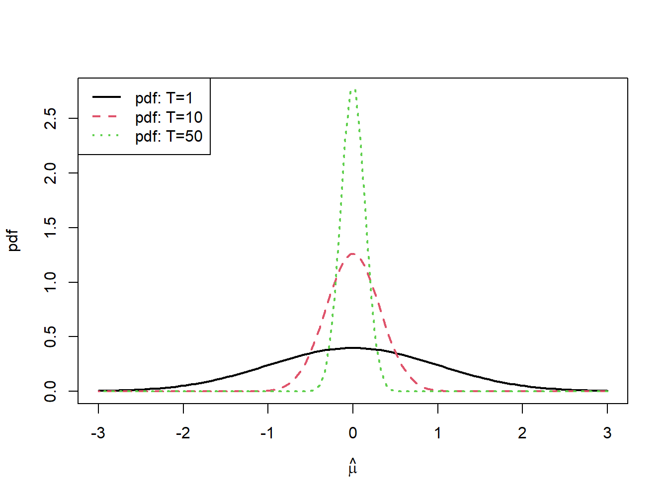
Figure 7.4: \(N(0,1/T)\) sampling distributions for \(\hat{\mu}\) for \(T=1,10\) and \(50\).
7.5.3.2 Confidence Intervals for \(\mu_{i}\)
In practice, the precision of \(\hat{\mu}_{i}\) is measured by \(\widehat{\mathrm{se}}(\hat{\mu}_{i})\) but is best communicated by computing a confidence interval for the unknown value of \(\mu_{i}\). A confidence interval is an interval estimate of \(\mu_{i}\) such that we can put an explicit probability statement about the likelihood that the interval covers \(\mu_{i}\).
Because we know the exact finite sample distribution of \(\hat{\mu}_{i}\) in the GWN return model, we can construct an exact confidence interval for \(\mu_{i}\).
Proposition 7.7 (t-ratio for sample mean) Let \(\{R_{it}\}_{t=1}^{T}\) be generated from the GWN model (7.1). Define the \(t\)-ratio as: \[\begin{equation} t_{i}=\frac{\hat{\mu}_{i}-\mu_{i}}{\widehat{\mathrm{se}}(\hat{\mu}_{i})}=\frac{\hat{\mu}_{i}-\mu_{i}}{\hat{\sigma}/\sqrt{T}},\tag{7.30} \end{equation}\] Then \(t_{i}\sim t_{T-1}\) where \(t_{T-1}\) denotes a Student’s \(t\) random variable with \(T-1\) degrees of freedom.
The Student’s \(t\) distribution with \(v>0\) degrees of freedom is a symmetric distribution centered at zero, like the standard normal. The tail-thickness (kurtosis) of the distribution is determined by the degrees of freedom parameter \(v\). For values of \(v\) close to zero, the tails of the Student’s \(t\) distribution are much fatter than the tails of the standard normal distribution. As \(v\) gets large, the Student’s \(t\) distribution approaches the standard normal distribution.
For \(\alpha\in(0,1)\), we compute a \((1-\alpha)\cdot100\%\) confidence interval for \(\mu_{i}\) using (7.30) and the \(1-\alpha/2\) quantile (critical value) \(t_{T-1}(1-\alpha/2)\) to give: \[ \Pr\left(-t_{T-1}(1-\alpha/2)\leq\frac{\hat{\mu}_{i}-\mu_{i}}{\widehat{\mathrm{se}}(\hat{\mu}_{i})}\leq t_{T-1}(1-\alpha/2)\right)=1-\alpha, \] which can be rearranged as, \[ \Pr\left(\hat{\mu}_{i}-t_{T-1}(1-\alpha/2)\cdot\widehat{\mathrm{se}}(\hat{\mu}_{i})\leq\mu_{i}\leq\hat{\mu}_{i}+t_{T-1}(1-\alpha/2)\cdot\widehat{\mathrm{se}}(\hat{\mu}_{i})\right)=1-\alpha. \] Hence, the interval, \[\begin{align} & [\hat{\mu}_{i}-t_{T-1}(1-\alpha/2)\cdot\widehat{\mathrm{se}}(\hat{\mu}_{i}),~\hat{\mu}_{i}+t_{T-1}(1-\alpha/2)\cdot\widehat{\mathrm{se}}(\hat{\mu}_{i})]\tag{7.31}\\ =& \hat{\mu}_{i}\pm t_{T-1}(1-\alpha/2)\cdot\widehat{\mathrm{se}}(\hat{\mu}_{i})\nonumber \end{align}\] covers the true unknown value of \(\mu_{i}\) with probability \(1-\alpha\).
Suppose we want to compute a 95% confidence interval for \(\mu_{i}\).
In this case \(\alpha=0.05\) and \(1-\alpha=0.95\). Suppose further
that \(T-1=60\) (e.g., five years of monthly return data) so that \(t_{T-1}(1-\alpha/2)=t_{60}(0.975)=2\).
This can be verified in R using the function qt().
Then the 95% confidence for \(\mu_{i}\) is given by:
\[\begin{equation} \hat{\mu}_{i}\pm2\cdot\widehat{\mathrm{se}}(\hat{\mu}_{i}).\tag{7.32} \end{equation}\]
The above formula for a 95% confidence interval is often used as a rule of thumb for computing an approximate 95% confidence interval for moderate sample sizes. It is easy to remember and does not require the computation of the quantile \(t_{T-1}(1-\alpha/2)\) from the Student’s \(t\) distribution. It is also an approximate 95% confidence interval that is based the asymptotic normality of \(\hat{\mu}_{i}\). Recall, for a normal distribution with mean \(\mu\) and variance \(\sigma^{2}\) approximately 95% of the probability lies between \(\mu\pm2\sigma\).
\(\blacksquare\)
The coverage probability associated with the confidence interval for \(\mu_{i}\) is based on the fact that the estimator \(\hat{\mu}_{i}\) is a random variable. Since the confidence interval is constructed as \(\hat{\mu}_{i}\pm t_{T-1}(1-\alpha/2)\cdot\widehat{\mathrm{se}}(\hat{\mu}_{i})\) it is also a random variable. An intuitive way to think about the coverage probability associated with the confidence interval is to think about the game of “horseshoes”37. The horseshoe is the confidence interval and the parameter \(\mu_{i}\) is the post at which the horse shoe is tossed. Think of playing the game 100 times. If the thrower is 95% accurate (if the coverage probability is 0.95) then 95 of the 100 tosses should ring the post (95 of the constructed confidence intervals should contain the true value \(\mu_{i})\).
Consider computing 95% confidence intervals for \(\mu_{i}\) using
(7.31) based on the estimated results for the Microsoft,
Starbucks and S&P 500 data. The degrees of freedom for the Student’s
\(t\) distribution is \(T-1=171\). The 97.5% quantile, \(t_{99}(0.975)\),
can be computed using the R function qt():
## [1] 1.97Notice that this quantile is very close to \(2.\) Then the exact 95% confidence intervals are given by:
lower = muhat - t.975*seMuhat
upper = muhat + t.975*seMuhat
width = upper - lower
ans= cbind(lower, upper, width)
colnames(ans) = c("2.5%", "97.5%", "Width")
ans
## 2.5% 97.5% Width
## MSFT -0.01096 0.01921 0.0302
## SBUX -0.00215 0.03146 0.0336
## SP500 -0.00561 0.00898 0.0146With probability 0.95, the above intervals will contain the true mean values assuming the GWN model is valid. The 95% confidence intervals for Microsoft and Starbucks are fairly wide (about 3%) and contain both negative and positive values. The confidence interval for the S&P 500 index is tighter but also contains negative and positive values. For Microsoft, the confidence interval is \([-1.1\%~1.9\%]\). This means that with probability 0.95, the true monthly expected return is somewhere between -1.1% and 1.9%. The economic implications of a -1.1% expected monthly return and a 1.9% expected return are vastly different. In contrast, the 95% confidence interval for the SP500 is about half the width of the intervals for Microsoft or Starbucks. The lower limit is near -0.5% and the upper limit is near 1%. This result clearly shows that the monthly mean return for the S&P 500 index is estimated much more precisely than the monthly mean returns for Microsoft or Starbucks.
7.5.3.3 Sampling Distributions for \(\hat{\sigma}_{i}^{2}\), \(\hat{\sigma}_{i}\), \(\hat{\sigma}_{ij}\), and \(\hat{\rho}_{ij}\)
The exact distributions of \(\hat{\sigma}_{i}^{2}\), \(\hat{\sigma}_{i}\), \(\hat{\sigma}_{ij}\), and \(\hat{\rho}_{ij}\) based on a fixed sample size \(T\) are not normal distributions and are difficult to derive38. However, approximate normal distributions of the form (7.7) based on the CLT are readily available:
\[\begin{align} & \hat{\sigma}_{i}^{2}\sim N\left(\sigma_{i}^{2},\widehat{\mathrm{se}}(\hat{\sigma}_{i}^{2})^{2}\right)=N\left(\sigma_{i}^{2},\frac{4\hat{\sigma}_{i}^{4}}{T}\right),\tag{7.33}\\ & \hat{\sigma}_{i}\sim N\left(\sigma_{i},\widehat{\mathrm{se}}(\hat{\sigma}_{i})^{2}\right)=N\left(\sigma_{i},\frac{\hat{\sigma}_{i}^{2}}{2T}\right),\tag{7.34}\\ & \hat{\sigma}_{ij} \sim N\left(\sigma_{ij},\widehat{\mathrm{se}}(\hat{\sigma}_{ij})^{2}\right)= N\left(\sigma_{ij}, \frac{\hat{\sigma}_i^2 \hat{\sigma}_j^2(1 + \hat{\rho}_{ij}^2)}{T} \right) \tag{7.35}\\ & \hat{\rho}_{ij}\sim N\left(\rho_{ij},\widehat{\mathrm{se}}(\hat{\rho}_{ij})^{2}\right)=N\left(\rho_{ij},\frac{(1-\hat{\rho}_{ij}^{2})^{2}}{T}\right).\tag{7.36} \end{align}\]
These approximate normal distributions can be used to compute approximate confidence intervals for \(\sigma_{i}^{2}\), \(\sigma_{i}\), \(\sigma_{ij}\) and \(\rho_{ij}\).
7.5.3.4 Approximate Confidence Intervals for \(\sigma_{i}^{2},\sigma_{i}\), \(\sigma_{ij}\), and \(\rho_{ij}\)
Approximate 95% confidence intervals for \(\sigma_{i}^{2},\sigma_{i}\) and \(\rho_{ij}\) are given by: \[\begin{align} \hat{\sigma}_{i}^{2}\pm2\cdot\widehat{\mathrm{se}}(\hat{\sigma}_{i}^{2}) & =\hat{\sigma}_{i}^{2}\pm2\cdot\frac{\hat{\sigma}_{i}^{2}}{\sqrt{T/2}},\tag{7.37}\\ \hat{\sigma}_{i}\pm2\cdot\widehat{\mathrm{se}}(\hat{\sigma}_{i}) & =\hat{\sigma}_{i}\pm2\cdot\frac{\hat{\sigma}_{i}}{\sqrt{2T}},\tag{7.38}\\ \hat{\sigma}_{ij}\pm2\cdot\widehat{\mathrm{se}}(\hat{\sigma}_{ij}) & = \hat{\sigma}_{ij}\pm2\cdot\frac{\sqrt{\hat{\sigma}_i^2 \hat{\sigma}_j^2(1+\hat{\rho}_{ij}^2)}}{\sqrt{T}}.\tag{7.39}\\ \hat{\rho}_{ij}\pm2\cdot\widehat{\mathrm{se}}(\hat{\rho}_{ij}) & =\hat{\rho}_{ij}\pm2\cdot\frac{(1-\hat{\rho}_{ij}^{2})}{\sqrt{T}}.\tag{7.40} \end{align}\]
Using (7.37) - (7.38), the approximate 95% confidence intervals for \(\sigma_{i}^{2}\) and \(\sigma_{i}\) (\(i=\) Microsoft, Starbucks, S&P 500) are:
# 95% confidence interval for variance
lowerSigma2 = sigma2hat - 2*seSigma2hat
upperSigma2 = sigma2hat + 2*seSigma2hat
widthSigma2 = upperSigma2 - lowerSigma2
ans = cbind(lowerSigma2, upperSigma2, widthSigma2)
colnames(ans) = c("2.5%", "97.5%", "Width")
ans
## 2.5% 97.5% Width
## MSFT 0.00788 0.01221 0.00433
## SBUX 0.00978 0.01515 0.00538
## SP500 0.00184 0.00286 0.00101# 95% confidence interval for volatility
lowerSigma = sigmahat - 2*seSigmahat
upperSigma = sigmahat + 2*seSigmahat
widthSigma = upperSigma - lowerSigma
ans = cbind(lowerSigma, upperSigma, widthSigma)
colnames(ans) = c("2.5%", "97.5%", "Width")
ans## 2.5% 97.5% Width
## MSFT 0.0894 0.1110 0.0216
## SBUX 0.0996 0.1237 0.0241
## SP500 0.0432 0.0537 0.0105The 95% confidence intervals for \(\sigma\) and \(\sigma^{2}\) are larger for Microsoft and Starbucks than for the S&P 500 index. For all assets, the intervals for \(\sigma\) are fairly narrow (2% for Microsoft and Starbucks and 1% for S&P 500 index) indicating that \(\sigma\) is precisely estimated.
The approximate 95% confidence intervals for \(\sigma_{ij}\) are:
lowerCov = covhat - 2*seCovhat
upperCov = covhat + 2*seCovhat
widthCov = upperCov - lowerCov
ans = cbind(lowerCov, upperCov, widthCov)
colnames(ans) = c("2.5%", "97.5%", "Width")
ans
## 2.5% 97.5% Width
## msft,sbux 0.00201 0.00562 0.00361
## msft,sp500 0.00213 0.00387 0.00174
## sbux,sp500 0.00157 0.00338 0.00181The approximate 95% confidence intervals for \(\rho_{ij}\) are:
lowerRho = rhohat - 2*seRhohat
upperRho = rhohat + 2*seRhohat
widthRho = upperRho - lowerRho
ans = cbind(lowerRho, upperRho, widthRho)
colnames(ans) = c("2.5%", "97.5%", "Width")
ans
## 2.5% 97.5% Width
## msft,sbux 0.206 0.476 0.270
## msft,sp500 0.523 0.712 0.189
## sbux,sp500 0.337 0.578 0.241The 95% confidence intervals for \(\sigma_{ij}\) \(\rho_{ij}\) are not too wide and all contain just positive values away from zero. The smallest interval is for \(\rho_{\textrm{msft,sp500}}\) because \(\hat{\rho}_{\textrm{msft,sp500}}\) is closest to 1.
\(\blacksquare\)
The matrix sample statistics (7.16) and (7.17) are unbiased estimators of \(\mu\) and \(\Sigma\), respectively.↩︎
Horse shoes is a game commonly played at county fairs. See (http://en.wikipedia.org/wiki/Horseshoes) for a complete description of the game.↩︎
For example, the exact sampling distribution of \((T-1)\hat{\sigma}_{i}^{2}/\sigma_{i}^{2}\) is chi-square with \(T-1\) degrees of freedom.↩︎