13.3 Portfolio Theory with Short Sales Constraints in a General Setting
In this section we extend the analysis of the previous section to the more general setting of \(N\) risky assets plus a risk free asset.
13.3.1 Multiple risky assets
The example data on Microsoft, Nordstrom and Starbucks from Chapter 12 is used to illustrate the computation of mean-variance efficient portfolios with short sales constraints. These data are created using:
asset.names <- c("MSFT", "NORD", "SBUX")
mu.vec = c(0.0427, 0.0015, 0.0285)
names(mu.vec) = asset.names
sigma.mat = matrix(c(0.0100, 0.0018, 0.0011,
           0.0018, 0.0109, 0.0026,
           0.0011, 0.0026, 0.0199),
         nrow=3, ncol=3)
dimnames(sigma.mat) = list(asset.names, asset.names)
sd.vec = sqrt(diag(sigma.mat))
r.f=0.005
The impact of the no short sales restrictions on the risk-return characteristics of feasible portfolios is nicely illustrated by constructing random long-only portfolios of these three assets:
set.seed(123)
x.msft = runif(400, min=0, max=1)
x.nord = runif(400, min=0, max=1)
x.sbux = 1 - x.msft - x.nord
long.only = which(x.sbux > 0)
x.msft = x.msft[long.only]
x.nord = x.nord[long.only]
x.sbux = x.sbux[long.only]
length(long.only)
## [1] 191Here we first create 400 random weights for Microsoft and Nordstrom that lie between zero and one, respectively. Then, we determine the weight on Starbucks and throw out portfolios for which the weight on Starbucks is negative. The remaining 191 portfolios are then long-only portfolios. To be sure, these weights are illustrated in Figure 13.6 created using:
library(PerformanceAnalytics)
chart.StackedBar(cbind(x.msft, x.nord, x.sbux),
                 main="Random long-only portfolio weight vectors",                             xlab = "portfolio", ylab = "weights",
                 xaxis.labels=as.character(1:length(long.only)))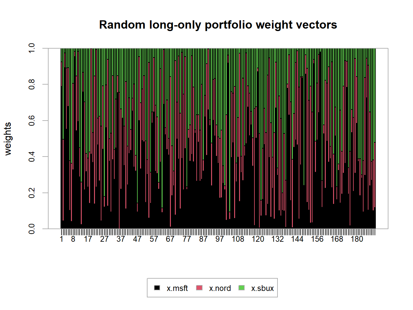
Figure 13.6: Weights on 191 random long-only portfolios of Microsoft, Nordstrom and Starbucks.
plot(sd.vec, mu.vec,  ylim=c(0, 0.05), xlim=c(0, 0.2),
     ylab=expression(mu[p]),
     xlab=expression(sigma[p]), type="n", cex.lab=1.5)
for (i in 1:length(long.only)) {
   z.vec = c(x.msft[i], x.nord[i], x.sbux[i])
   mu.p = crossprod(z.vec,mu.vec)
   sig.p = sqrt(t(z.vec)%*%sigma.mat%*%z.vec)
   points(sig.p, mu.p, pch=16, col="grey", cex=1.5)
}
points(sd.vec, mu.vec, pch=16, col="black", cex=2.5, cex.lab=1.75)
text(sd.vec, mu.vec, labels=asset.names, pos=4, cex = cex.val)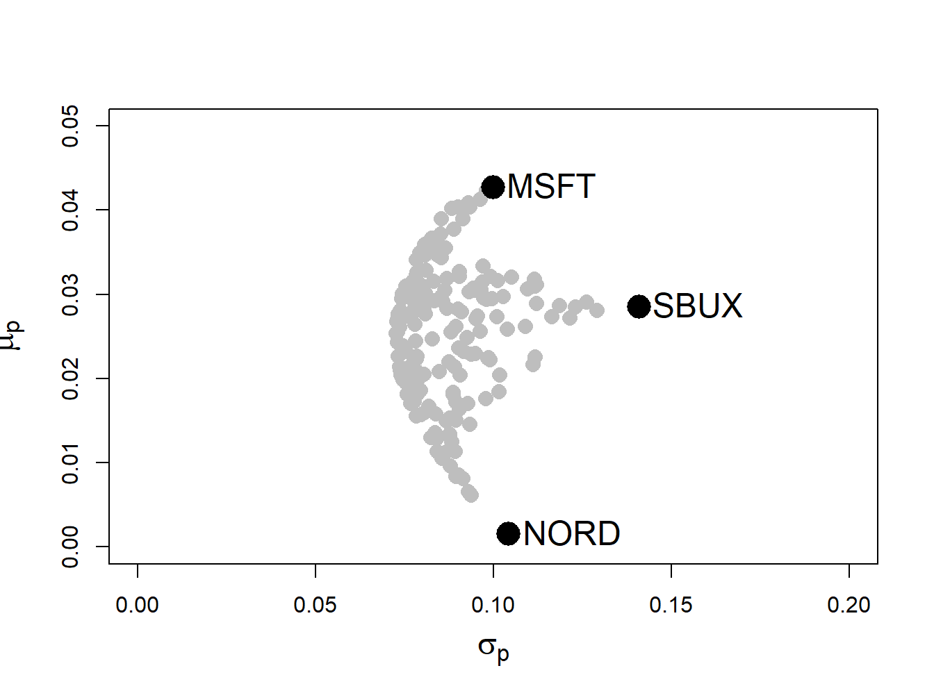
Figure 13.7: Risk-return characteristics of 191 random long-only portfolios of Microsoft, Nordstrom and Starbucks.
The shape of the risk-return scatter is revealing. No random long-only portfolio has an expected return higher than the expected return on Microsoft, which is the asset with the highest expected return. Similarly, no random portfolio has an expected return lower than the expected return on Nordstrom - which is the asset with the lowest expected return. Finally, no random portfolio has a volatility higher than the volatility on Starbucks, the asset with the highest volatility. The scatter of points has a convex (to the origin) parabolic-shaped outer boundary with endpoints at Microsoft and Nordstrom, respectively. The points inside the boundary taper outward from Starbucks towards the outer boundary. The entire risk-return scatter resembles an umbrella tipped on its side with spires extending from the outer boundary to the individual assets.
13.3.2 Portfolio optimization imposing no-short sales constraints
Consider an investment universe with \(N\) risky assets whose simple returns are described by the GWN model with expected return vector \(\mu\) and covariance matrix \(\Sigma\). The optimization problem to solve for the global minimum variance portfolio \(\mathbf{m}\) with no-short sales constraints on all assets is a straightforward extension of the problem that allows short sales. We simply add the \(N\) no-short sales inequality constraints \(m_{i}\geq0\,(i=1,\ldots,N)\). The optimization problem is: \[\begin{align} \min_{\mathbf{m}}\sigma_{p,m}^{2} & =\mathbf{m}^{\prime}\Sigma \mathbf{m}\tag{13.2}\\ \text{s.t. } \mathbf{m}^{\prime}\mathbf{1} & =1,\nonumber \\ m_{i} & \geq0\text{ }(i=1,\ldots,N).\nonumber \end{align}\] Here, there is one equality constraint, \(\mathbf{m}^{\prime}\mathbf{1}=1\), and \(N\) inequality constraints, \(m_{i}\geq0\text{ }(i=1,\ldots,N)\).
Similarly, the optimization problem to solve for a minimum variance portfolio \(\mathbf{x}\) with target expected return \(\mu_{p}^{0}\) and no short sales allowed for any asset becomes: \[\begin{align} \min_{\mathbf{x}}\sigma_{p,x}^{2} & =\mathbf{x}^{\prime}\Sigma \mathbf{x} \tag{13.3}\\ \text{s.t. }\mu_{p,x} & =\mathbf{x}^{\prime}\mu=\mu_{p}^{0},\nonumber \\ \mathbf{x}^{\prime}\mathbf{1} & =1,\nonumber \\ x_{i} & \geq0\text{ }(i=1,\ldots,N).\nonumber \end{align}\] Here there are two equality constraints, \(\mathbf{x}^{\prime}\mu=\mu_{p}^{0}\) and \(\mathbf{x}^{\prime}\mathbf{1}=1\), and \(N\) inequality constraints, \(x_{i}\geq0\text{ }(i=1,\ldots,N)\)
Remarks:
- The optimization problems (13.2) and (13.3), unfortunately, cannot be analytically solved using the method of Lagrange multipliers due to the inequality constraints. They must be solved numerically using an optimization algorithm. Fortunately, the optimization problems (13.2) and (13.3) are special cases of a more general quadratic programming problem for which there is a specialized optimization algorithm that is fast and efficient and available in R in the package quadprog.89
- There may not be a feasible solution to (13.3). That is, there may not exist a no-short sale portfolio \(\mathbf{x}\) that reaches the target return \(\mu_{p}^{0}.\) For example, in Figure 13.7 there is no efficient portfolio that has target expected return higher than the expected return on Microsoft. In general, with \(N\) assets there is no feasible solution to (13.3) for target expected returns higher than the maximum expected return among the \(N\) assets. If you try to solve (13.3) for an infeasible target expected return, the numerical optimizer will return an error message that indicates no solution is found.
- The portfolio variances associated with the solutions to (13.2) and (13.3), respectively, must be at least as large as the variances associated with the solutions that do not impose the short sales restrictions. Intuitively this makes sense. Adding additional constraints to a minimization problem will lead to a higher minimum at the solution if the additional constraints are binding. If the constraints are not binding, then the solution with and without the additional constraints are the same.
- The entire frontier of minimum variance portfolios without short sales exists only for target expected returns between the expected return on the global minimum variance portfolio with no short sales that solves (13.2) and the target expected return equal to the maximum expected return among the \(N\) assets. For these target returns, the no-short sales frontier will lie inside and to the right of the frontier that allows short sales if the no-short sales restrictions are binding for some asset.
- The entire frontier of minimum variance portfolios without short sales can no longer be constructed from any two frontier portfolios. It has to be computed by brute force for each portfolio solving (13.3) with target expected return \(\mu_{p}^{0}\) above the expected return on the the global minimum variance portfolio that solves (13.2) and below the target return equal to the maximum expected return among the \(N\) assets.
See the CRAN Optimization Task View for additional R packages that can be used to solve QP problems.↩︎