16.3 Monte Carlo Simulation of the SI Model

To give a first step reality check for the SI model, consider simulating data from the SI model for a single asset. The steps to create a Monte Carlo simulation from the SI model are:

1. Fix values for the SI model parameters $\alpha$, $\beta$, $\sigma_{\epsilon}$, $\mu_{M}$ and $\sigma_{M}$
2. Determine the number of simulated returns, $T$, to create.
3. Use a computer random number generator to simulate $T$ iid values of $R_{Mt}\sim N(\mu_{M},\sigma_{M}^{2})$ and $\epsilon_{t}\sim N(0,\sigma_{\epsilon}^{2})$, where $R_{Mt}$ is simulated independently from $\epsilon_{t}$.
4. Create the simulated asset returns $\tilde{R}_{t}=\alpha+\beta\tilde{R}_{M}$+$\tilde{\epsilon}_{t}$ for $t=1,\ldots,T$

The following example illustrates simulating SI model returns for Boeing.

Example 4.3 (Simulating monthly returns from the SI model for Boeing)

Consider simulating monthly returns on Boeing from the SI model where the S&P 500 index is used as the market index. The SI model parameters are calibrated from the actual monthly returns on Boeing and the S&P 500 index using sample statistics, as discussed in the next section, and are given by: $$\alpha_{BA}=0.005,\,\beta_{BA}=0.98,\,\sigma_{\epsilon,BA}=0.08,\,\mu_{M}=0.003,\,\sigma_{M}=0.048.$$ These values are set in R using:

alpha.BA = 0.005 
beta.BA = 0.98 
sd.e.BA = 0.08 
mu.sp500 = 0.003 
sd.sp500 = 0.048

The simulated returns for the S&P 500 index and Boeing are created using:

n.sim = nrow(siRetS) 
set.seed(123) 
sp500.sim = rnorm(n.sim, mu.sp500, sd.sp500) 
e.BA.sim = rnorm(n.sim, 0, sd.e.BA) 
BA.sim = alpha.BA + beta.BA*sp500.sim + e.BA.sim 
BA.sim = xts(BA.sim, index(siRetS)) 
sp500.sim = xts(sp500.sim, index(siRetS)) 
colnames(BA.sim) = "BA.sim" 
colnames(sp500.sim) = "SP500.sim"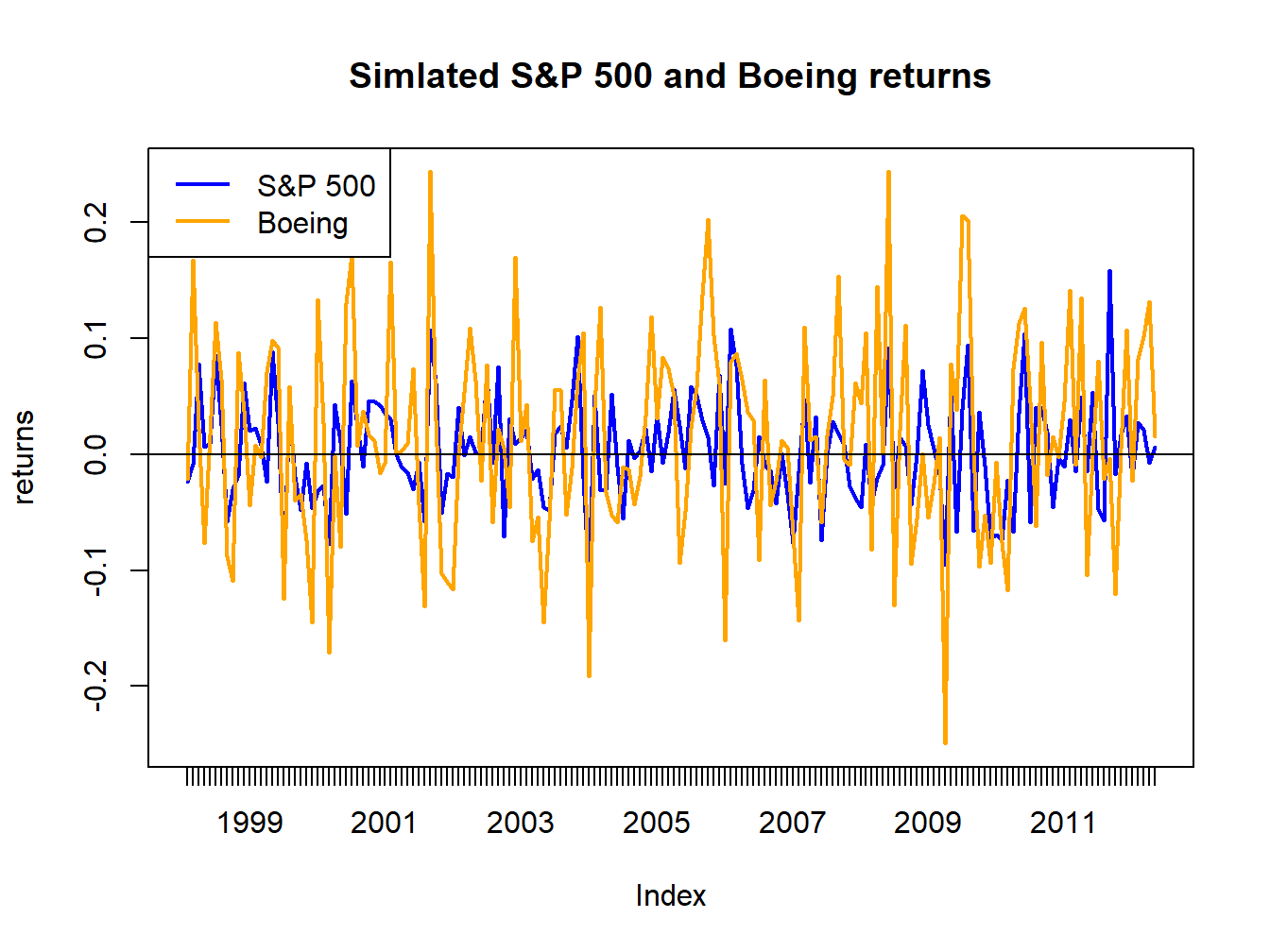

Figure 16.5: Simulated SI model monthly returns on the S&P 500 index and Boeing.

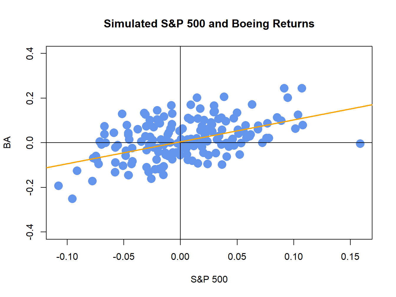
Figure 16.6: Simulated SI model monthly returns on the S&P 500 index and Boeing. The orange line is the equation $R_{BA,t}=\alpha_{BA}+\beta_{BA}R_{Mt}=0.005+0.98\times R_{Mt}.$

The simulate returns are illustrated in Figures 16.5 and 16.6. The time plot and scatterplot of the simulated returns on the S&P 500 index look much like the corresponding plots of the actual returns shows in the top left panels of Figures 16.2 and 16.4, respectively. Hence, the SI model for the S&P 500 index and Boeing passes the first step reality check. In Figure 16.6, the line $\alpha_{i}+\beta_{i}R_{Mt}=0.005+0.98R_{Mt}$ is shown in orange. This line represents the predictions of Boeing’s return given the S&P 500 return. For example, if $R_{Mt}=0.05$ then the predicted return for Boeing is $R_{BA}=0.005+0.98\times(0.05)=0.054$. The differences between the observed Boeing returns and (blue dots) and the predicted returns (orange line) are the asset specific error terms. These are the random asset specific news components. The standard deviation of these components, $\sigma_{\epsilon,BA}=0.08$, represents the typical magnitude of these components. Here, we would not be too surprised if the observed Boeing return is $0.08$ above or below the orange line. How close the Boeing returns are to the predicted returns is determined by the $R^{2}$ value given by (16.15). Here, $\sigma_{BA}^{2}=\beta_{BA}^{2}\sigma_{M}^{2}+\sigma_{\epsilon,BA}^{2}=(0.98)^{2}(0.048)^{2}+(0.08)^{2}=0.00861$ and so $R^{2}=(0.98)^{2}(0.048)^{2}/0.00861=0.257$. Hence, 25.7% of the variability (risk) of Boeing returns are explained by the variability of the S&P 500 returns. As a result, 74.3% $(1-R^{2}=0.743)$ of the variability of Boeing returns are due to the random asset specific terms.

$\blacksquare$