3.4 Systems of Linear Equations
Consider the system of two linear equations: \[\begin{align} x+y & =1,\tag{3.1}\\ 2x-y & =1.\tag{3.2} \end{align}\] As shown in Figure 3.1, equations (3.1) and (3.2) represent two straight lines which intersect at the point \(x=2/3\) and \(y=1/3\). This point of intersection is determined by solving for the values of \(x\) and \(y\) such that \(x+y=2x-y\)14
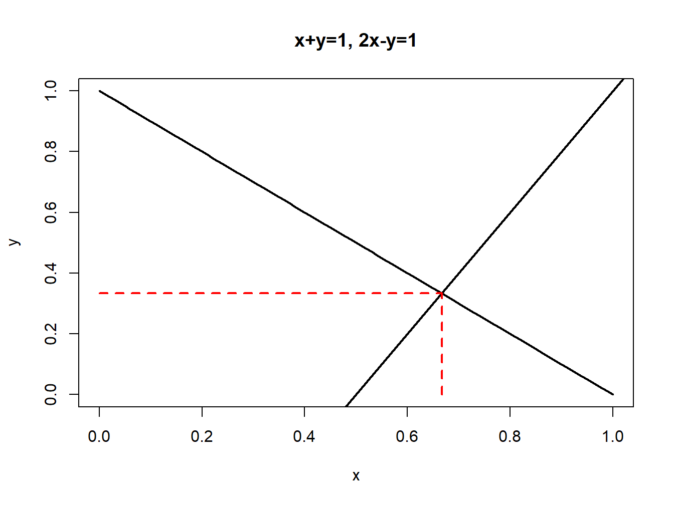
Figure 3.1: System of two linear equations.
The two linear equations can be written in matrix form as: \[ \left[\begin{array}{cc} 1 & 1\\ 2 & -1 \end{array}\right]\left[\begin{array}{c} x\\ y \end{array}\right]=\left[\begin{array}{c} 1\\ 1 \end{array}\right], \] or, \[ \mathbf{A\cdot z=b,} \] where, \[ \mathbf{A}=\left[\begin{array}{cc} 1 & 1\\ 2 & -1 \end{array}\right],~\mathbf{z}=\left[\begin{array}{c} x\\ y \end{array}\right]\textrm{ and }\mathbf{b}=\left[\begin{array}{c} 1\\ 1 \end{array}\right]. \]
If there was a \((2\times2)\) matrix \(\mathbf{B},\) with elements \(b_{ij}\), such that \(\mathbf{B\cdot A=I}_{2},\) where \(\mathbf{I}_{2}\) is the \((2\times2)\) identity matrix, then we could solve for the elements in \(\mathbf{z}\) as follows. In the equation \(\mathbf{A\cdot z=b}\), pre-multiply both sides by \(\mathbf{B}\) to give: \[\begin{align*} \mathbf{B\cdot A\cdot z} & =\mathbf{B\cdot b}\\ & \Longrightarrow\mathbf{I\cdot z=B\cdot b}\\ & \Longrightarrow\mathbf{z=B\cdot b}, \end{align*}\] or \[ \left[\begin{array}{c} x\\ y \end{array}\right]=\left[\begin{array}{cc} b_{11} & b_{12}\\ b_{21} & b_{22} \end{array}\right]\left[\begin{array}{c} 1\\ 1 \end{array}\right]=\left[\begin{array}{c} b_{11}\cdot1+b_{12}\cdot1\\ b_{21}\cdot1+b_{22}\cdot1 \end{array}\right]. \] If such a matrix \(\mathbf{B}\) exists it is called the inverse of \(\mathbf{A}\) and is denoted \(\mathbf{A}^{-1}\). Intuitively, the inverse matrix \(\mathbf{A}^{-1}\) plays a similar role as the inverse of a number. Suppose \(a\) is a number; e.g., \(a=2\). Then we know that \((1/a)\cdot a=a^{-1}a=1\). Similarly, in matrix algebra \(\mathbf{A}^{-1}\mathbf{A=I}_{2}\) where \(\mathbf{I}_{2}\) is the identity matrix. Now, consider solving the equation \(a\cdot x=b\). By simple division we have that \(x=(1/a)\cdot b=a^{-1}\cdot b\). Similarly, in matrix algebra, if we want to solve the system of linear equations \(\mathbf{Ax=b}\) we pre-multiply by \(\mathbf{A}^{-1}\) and get the solution \(\mathbf{x=A}^{-1}\mathbf{b}\).
Using \(\mathbf{B=A}^{-1}\), we may express the solution for \(\mathbf{z}\) as: \[ \mathbf{z=A}^{-1}\mathbf{b}. \] As long as we can determine the elements in \(\mathbf{A}^{-1}\) then we can solve for the values of \(x\) and \(y\) in the vector \(\mathbf{z}\). The system of linear equations has a solution as long as the two lines intersect, so we can determine the elements in \(\mathbf{A}^{-1}\) provided the two lines are not parallel. If the two lines are parallel, then one of the equations is a multiple of the other. In this case, we say that \(\mathbf{A}\) is not invertible.
There are general numerical algorithms for finding the elements of \(\mathbf{A}^{-1}\) (e.g., Gaussian elimination) and R has these algorithms available. However, if \(\mathbf{A}\) is a \((2\times2)\) matrix then there is a simple formula for \(\mathbf{A}^{-1}\). Let \(\mathbf{A}\) be a \((2\times2)\) matrix such that: \[ \mathbf{A}=\left[\begin{array}{cc} a_{11} & a_{12}\\ a_{21} & a_{22} \end{array}\right]. \] Then, \[ \mathbf{A}^{-1}=\frac{1}{\det(\mathbf{A})}\left[\begin{array}{cc} a_{22} & -a_{12}\\ -a_{21} & a_{11} \end{array}\right], \] where \(\det(\mathbf{A})=a_{11}a_{22}-a_{21}a_{12}\) denotes the determinant of \(\mathbf{A}\) and is assumed to be not equal to zero. By brute force matrix multiplication we can verify this formula: \[\begin{align*} \mathbf{A}^{-1}\mathbf{A} & =\frac{1}{a_{11}a_{22}-a_{21}a_{12}}\left[\begin{array}{cc} a_{22} & -a_{12}\\ -a_{21} & a_{11} \end{array}\right]\left[\begin{array}{cc} a_{11} & a_{12}\\ a_{21} & a_{22} \end{array}\right]\\ & =\frac{1}{a_{11}a_{22}-a_{21}a_{12}}\left[\begin{array}{cc} a_{22}a_{11}-a_{12}a_{21} & a_{22}a_{12}-a_{12}a_{22}\\ -a_{21}a_{11}+a_{11}a_{21} & -a_{21}a_{12}+a_{11}a_{22} \end{array}\right]\\ & =\frac{1}{a_{11}a_{22}-a_{21}a_{12}}\left[\begin{array}{cc} a_{22}a_{11}-a_{12}a_{21} & 0\\ 0 & -a_{21}a_{12}+a_{11}a_{22} \end{array}\right]\\ & =\left[\begin{array}{cc} \dfrac{a_{22}a_{11}-a_{12}a_{21}}{a_{11}a_{22}-a_{21}a_{12}} & 0\\ 0 & \dfrac{-a_{21}a_{12}+a_{11}a_{22}}{a_{11}a_{22}-a_{21}a_{12}} \end{array}\right]\\ & =\left[\begin{array}{cc} 1 & 0\\ 0 & 1 \end{array}\right]. \end{align*}\] Let’s apply the above rule to find the inverse of \(\mathbf{A}\) in our example linear system (3.1)-(3.2): \[ \mathbf{A}^{-1}=\frac{1}{-1-2}\left[\begin{array}{cc} -1 & -1\\ -2 & 1 \end{array}\right]=\left[\begin{array}{cc} \frac{1}{3} & \frac{1}{3}\\ \frac{2}{3} & \frac{-1}{3} \end{array}\right]. \] Notice that, \[ \mathbf{A}^{-1}\mathbf{A}=\left[\begin{array}{cc} \frac{1}{3} & \frac{1}{3}\\ \frac{2}{3} & \frac{-1}{3} \end{array}\right]\left[\begin{array}{cc} 1 & 1\\ 2 & -1 \end{array}\right]=\left[\begin{array}{cc} 1 & 0\\ 0 & 1 \end{array}\right]. \] Our solution for \(\mathbf{z}\) is then, \[\begin{align*} \mathbf{z} & =\mathbf{A}^{-1}\mathbf{b}\\ & =\left[\begin{array}{cc} \frac{1}{3} & \frac{1}{3}\\ \frac{2}{3} & \frac{-1}{3} \end{array}\right]\left[\begin{array}{c} 1\\ 1 \end{array}\right]\\ & =\left[\begin{array}{c} \frac{2}{3}\\ \frac{1}{3} \end{array}\right]=\left[\begin{array}{c} x\\ y \end{array}\right], \end{align*}\] so that \(x=2/3\) and \(y=1/3\).
In R, the solve() function is used to compute the inverse
of a matrix and solve a system of linear equations. The linear system
\(x+y=1\) and \(2x-y=1\) can be represented using:
First we solve for \(\mathbf{A}^{-1}\):15
##           [,1]       [,2]
## [1,] 0.3333333  0.3333333
## [2,] 0.6666667 -0.3333333## [,1] [,2]
## [1,] 1 -5.551115e-17
## [2,] 0 1.000000e+00## [,1] [,2]
## [1,] 1 5.551115e-17
## [2,] 0 1.000000e+00Then we solve the system \(\mathbf{z}=\mathbf{A}^{-1}\mathbf{b}\):
##           [,1]
## [1,] 0.6666667
## [2,] 0.3333333
\(\blacksquare\)
In general, if we have \(n\) linear equations in \(n\) unknown variables we may write the system of equations as \[\begin{align*} a_{11}x_{1}+a_{12}x_{2}+\cdots+a_{1n}x_{n} & =b_{1}\\ a_{21}x_{1}+a_{22}x_{2}+\cdots+a_{2n}x_{n} & =b_{2}\\ \vdots & =\vdots\\ a_{n1}x_{1}+a_{n2}x_{2}+\cdots+a_{nn}x_{n} & =b_{n} \end{align*}\] which we may then express in matrix form as \[ \left[\begin{array}{cccc} a_{11} & a_{12} & \cdots & a_{1n}\\ a_{21} & a_{22} & \cdots & a_{2n}\\ \vdots & \vdots & \ddots & \vdots\\ a_{n1} & a_{n2} & \cdots & a_{nn} \end{array}\right]\left[\begin{array}{c} x_{1}\\ x_{2}\\ \vdots\\ x_{n} \end{array}\right]=\left[\begin{array}{c} b_{1}\\ b_{2}\\ \vdots\\ b_{n} \end{array}\right] \] or \[ \underset{(n\times n)}{\mathbf{A}}\cdot\underset{(n\times1)}{\mathbf{x}}=\underset{(n\times1)}{\mathbf{b}}. \] The solution to the system of equations is given by: \[ \mathbf{x=A}^{-1}\mathbf{b}, \] where \(\mathbf{A}^{-1}\mathbf{A}=\mathbf{I}_n\) and \(\mathbf{I}_{n}\) is the \((n\times n)\) identity matrix. If the number of equations is greater than two, then we generally use numerical algorithms to find the elements in \(\mathbf{A}^{-1}\).
3.4.1 Rank of a matrix
A \(n\times m\) matrix \(\mathbf{A}\) has \(m\) columns \(\mathbf{a}_{1},\mathbf{a}_{2},\ldots,\mathbf{a}_{m}\) where each column is an \(n\times1\) vector and \(n\) rows where each row is an \(1\times m\) row vector: \[ \underset{(n\times m)}{\mathbf{A}}=\left[\begin{array}{cccc} a_{11} & a_{12} & \ldots & a_{1m}\\ a_{21} & a_{22} & \ldots & a_{2m}\\ \vdots & \vdots & \ddots & \vdots\\ a_{n1} & a_{n2} & \ldots & a_{nm} \end{array}\right]=\left[\begin{array}{cccc} \mathbf{a}_{1} & \mathbf{a}_{2} & \ldots & \mathbf{a}_{m}\end{array}\right]. \] Two vectors \(\mathbf{a}_{1}\) and \(\mathbf{a}_{2}\) are linearly independent if \(c_{1}\mathbf{a}_{1}+c_{2}\mathbf{a}_{2}=0\) implies that \(c_{1}=c_{2}=0\). A set of vectors \(\mathbf{a}_{1},\mathbf{a}_{2},\ldots,\mathbf{a}_{m}\) are linearly independent if \(c_{1}\mathbf{a}_{1}+c_{2}\mathbf{a}_{2}+\cdots+c_{m}\mathbf{a}_{m}=0\) implies that \(c_{1}=c_{2}=\cdots=c_{m}=0\). That is, no vector \(\mathbf{a}_{i}\) can be expressed as a non-trivial linear combination of the other vectors.
The column rank of the \(n\times m\) matrix \(\mathbf{A}\), denoted \(\mathrm{rank}(\mathbf{A})\), is equal to the maximum number of linearly independent columns. The row rank of a matrix is equal to the maximum number of linearly independent rows, and is given by \(\mathrm{rank}(\mathbf{A}^{\prime})\). It turns out that the column rank and row rank of a matrix are the same. Hence, \(\mathrm{rank}(\mathbf{A})\)\(=\mathrm{rank}(\mathbf{A}^{\prime})\leq\mathrm{min}(m,n)\). If \(\mathrm{rank}(\mathbf{A})=m\) then \(\mathbf{A}\) is called full column rank, and if \(\mathrm{rank}(\mathbf{A})=n\) then \(\mathbf{A}\) is called full row rank. If \(\mathbf{A}\) is not full rank then it is called reduced rank.
Consider the \(2\times3\) matrix
\[
\mathbf{A}=\left(\begin{array}{ccc}
1 & 3 & 5\\
2 & 4 & 6
\end{array}\right)
\]
Here, \(\mathrm{rank}(\mathbf{A})\leq min(3,2)=2\), the number of rows.
Now, \(\mathrm{rank}(\mathbf{A})=2\) since the rows of \(\mathbf{A}\)
are linearly independent. In R, the rank of a matrix can be found
using the Matrix function rankMatrix():
## [1] 2\(\blacksquare\)
The rank of an \(n\times n\) square matrix \(\mathbf{A}\) is directly related to its invertibility. If \(\mathrm{rank}(\mathbf{A})=n\) then \(\mathbf{A}^{-1}\) exists. This result makes sense. Since \(\mathbf{A}^{-1}\) is used to solve a system of \(n\) linear equations in \(n\) unknowns, it will have a unique solution as long as no equation in the system can be written as a linear combination of the other equations.
3.4.2 Partitioned matrices and partitioned inverses
Consider a general \(n\times m\) matrix \(\mathbf{A}\): \[ \underset{(n\times m)}{\mathbf{A}}=\left[\begin{array}{cccc} a_{11} & a_{12} & \ldots & a_{1m}\\ a_{21} & a_{22} & \ldots & a_{2m}\\ \vdots & \vdots & \ddots & \vdots\\ a_{n1} & a_{n2} & \ldots & a_{nm} \end{array}\right]. \] In some situations we might want to partition \(\mathbf{A}\) into sub-matrices containing sub-blocks of the elements of \(\mathbf{A}\): \[ \mathbf{A}=\left[\begin{array}{cc} \mathbf{A}_{11} & \mathbf{A}_{12}\\ \mathbf{A}_{21} & \mathbf{A}_{22} \end{array}\right], \] where the sub-matrices \(\mathbf{A}_{11}\), \(\mathbf{A}_{12}\), \(\mathbf{A}_{21}\), and \(\mathbf{A}_{22}\) contain the appropriate sub-elements of \(\mathbf{A}\). For example, consider \[ \mathbf{A}=\left[\begin{array}{cc|cc} 1 & 2 & 3 & 4\\ 5 & 6 & 7 & 8\\ \hline 9 & 10 & 11 & 12\\ 13 & 14 & 15 & 16 \end{array}\right]=\left[\begin{array}{cc} \mathbf{A}_{11} & \mathbf{A}_{12}\\ \mathbf{A}_{21} & \mathbf{A}_{22} \end{array}\right], \] where \[\begin{eqnarray*} \mathbf{A}_{11} & = & \left[\begin{array}{cc} 1 & 2\\ 5 & 6 \end{array}\right],\,\mathbf{A}_{12}=\left[\begin{array}{cc} 3 & 4\\ 7 & 8 \end{array}\right],\\ \mathbf{A}_{21} & = & \left[\begin{array}{cc} 9 & 10\\ 13 & 14 \end{array}\right],\,\mathbf{A}_{22}=\left[\begin{array}{cc} 11 & 12\\ 15 & 16 \end{array}\right]. \end{eqnarray*}\]
In R sub-matrices can be combined column-wise using cbind(),
and row-wise using rbind(). For example, to create the matrix
\(\mathbf{A}\) from the sub-matrices use
A11mat = matrix(c(1,2,5,6), 2, 2, byrow=TRUE)
A12mat = matrix(c(3,4,7,8), 2, 2, byrow=TRUE)
A21mat = matrix(c(9,10,13,14), 2, 2, byrow=TRUE)
A22mat = matrix(c(11,12,15,16), 2, 2, byrow=TRUE)
Amat = rbind(cbind(A11mat, A12mat), cbind(A21mat, A22mat))
Amat
## [,1] [,2] [,3] [,4]
## [1,] 1 2 3 4
## [2,] 5 6 7 8
## [3,] 9 10 11 12
## [4,] 13 14 15 16\(\blacksquare\)
The basic matrix operations work on sub-matrices in the obvious way. To illustrate, consider another matrix \(\mathbf{B}\) that is conformable with \(\mathbf{A}\) and partitioned in the same way: \[ \mathbf{B}=\left[\begin{array}{cc} \mathbf{B}_{11} & \mathbf{B}_{12}\\ \mathbf{B}_{21} & \mathbf{B}_{22} \end{array}\right]. \] Then \[ \mathbf{A}+\mathbf{B}=\left[\begin{array}{cc} \mathbf{A}_{11} & \mathbf{A}_{12}\\ \mathbf{A}_{21} & \mathbf{A}_{22} \end{array}\right]+\left[\begin{array}{cc} \mathbf{B}_{11} & \mathbf{B}_{12}\\ \mathbf{B}_{21} & \mathbf{B}_{22} \end{array}\right]=\left[\begin{array}{cc} \mathbf{A}_{11}+\mathbf{B}_{11} & \mathbf{A}_{12}+\mathbf{B}_{12}\\ \mathbf{A}_{21}+\mathbf{B}_{21} & \mathbf{A}_{22}+\mathbf{B}_{22} \end{array}\right]. \] If all of the sub-matrices of \(\mathbf{A}\) and \(\mathbf{B}\) are comformable then \[ \mathbf{AB}=\left[\begin{array}{cc} \mathbf{A}_{11} & \mathbf{A}_{12}\\ \mathbf{A}_{21} & \mathbf{A}_{22} \end{array}\right]\left[\begin{array}{cc} \mathbf{B}_{11} & \mathbf{B}_{12}\\ \mathbf{B}_{21} & \mathbf{B}_{22} \end{array}\right]=\left[\begin{array}{cc} \mathbf{A}_{11}\mathbf{B}_{11}+\mathbf{A}_{12}\mathbf{B}_{21} & \mathbf{A}_{11}\mathbf{B}_{12}+\mathbf{A}_{12}\mathbf{B}_{22}\\ \mathbf{A}_{21}\mathbf{B}_{11}+\mathbf{A}_{22}\mathbf{B}_{21} & \mathbf{A}_{21}\mathbf{B}_{12}+\mathbf{A}_{22}\mathbf{B}_{22} \end{array}\right]. \]
The transpose of a partitioned matrix satisfies \[ \mathbf{A^{\prime}}=\left[\begin{array}{cc} \mathbf{A}_{11} & \mathbf{A}_{12}\\ \mathbf{A}_{21} & \mathbf{A}_{22} \end{array}\right]^{\prime}=\left[\begin{array}{cc} \mathbf{A}_{11}^{\prime} & \mathbf{A}_{21}^{\prime}\\ \mathbf{A}_{12}^{\prime} & \mathbf{A}_{22}^{\prime} \end{array}\right]. \] Notice the interchange of the two off-diagonal blocks.
A partitioned matrix \(\mathbf{A}\) with appropriate invertible sub-matrices \(\mathbf{A}_{11}\) and \(\mathbf{A}_{22}\) has a partitioned inverse of the form \[ \mathbf{A}^{-1}=\left[\begin{array}{cc} \mathbf{A}_{11} & \mathbf{A}_{12}\\ \mathbf{A}_{21} & \mathbf{A}_{22} \end{array}\right]^{-1}=\left[\begin{array}{cc} \mathbf{A}_{11}^{-1}+\mathbf{A}_{11}^{-1}\mathbf{A}_{12}\mathbf{C}^{-1}\mathbf{A}_{21}\mathbf{A}_{11}^{-1} & -\mathbf{A}_{11}\mathbf{A}_{12}\mathbf{C}^{-1}\\ -\mathbf{C}^{-1}\mathbf{A}_{21}\mathbf{A}_{11}^{-1} & \mathbf{C}^{-1} \end{array}\right], \] where \(\mathbf{C}=\mathbf{A}_{22}-\mathbf{A}_{21}\mathbf{A}_{11}^{-1}\mathbf{A}_{12}\). This formula can be verified by direct calculation.
Soving for \(x\) gives \(x=2y\). Substituting this value into the equation \(x+y=1\) gives \(2y+y=1\) and solving for \(y\) gives \(y=1/3\). Solving for \(x\) then gives \(x=2/3\).↩︎
Notice that the calculations in R do not show \(\mathbf{A}^{-1}\mathbf{A}=\mathbf{I}\) exactly. The (1,2) element of \(\mathbf{A}^{-1}\mathbf{A}\) is -5.552e-17, which for all practical purposes is zero. However, due to the limitations of machine calculations the result is not exactly zero.↩︎