5.3 Bivariate Descriptive
In this section, we consider graphical and numerical descriptive statistics for summarizing two or more data series.
5.3.1 Scatterplots
The contemporaneous dependence properties between two data series \(\{x_{t}\}_{t=1}^{T}\) and \(\{y_{t}\}_{t=1}^{T}\) can be displayed graphically in a scatterplot, which is simply an xy-plot of the bivariate data.
Figure 5.25 shows the scatterplots between the Microsoft and S&P 500 monthly and daily returns created using:
par(mfrow=c(1,2))
plot(coredata(sp500MonthlyRetS),coredata(msftMonthlyRetS),
     main="Monthly returns", xlab="S&P500", ylab="MSFT", lwd=2,
     pch=16, cex=1.25, col="blue")
abline(v=mean(sp500MonthlyRetS))
abline(h=mean(msftMonthlyRetS))
plot(coredata(sp500DailyRetS),coredata(msftDailyRetS),
     main="Daily returns", xlab="S&P500", ylab="MSFT", lwd=2,
     pch=16, cex=1.25, col="blue")
abline(v=mean(sp500DailyRetS))
abline(h=mean(msftDailyRetS))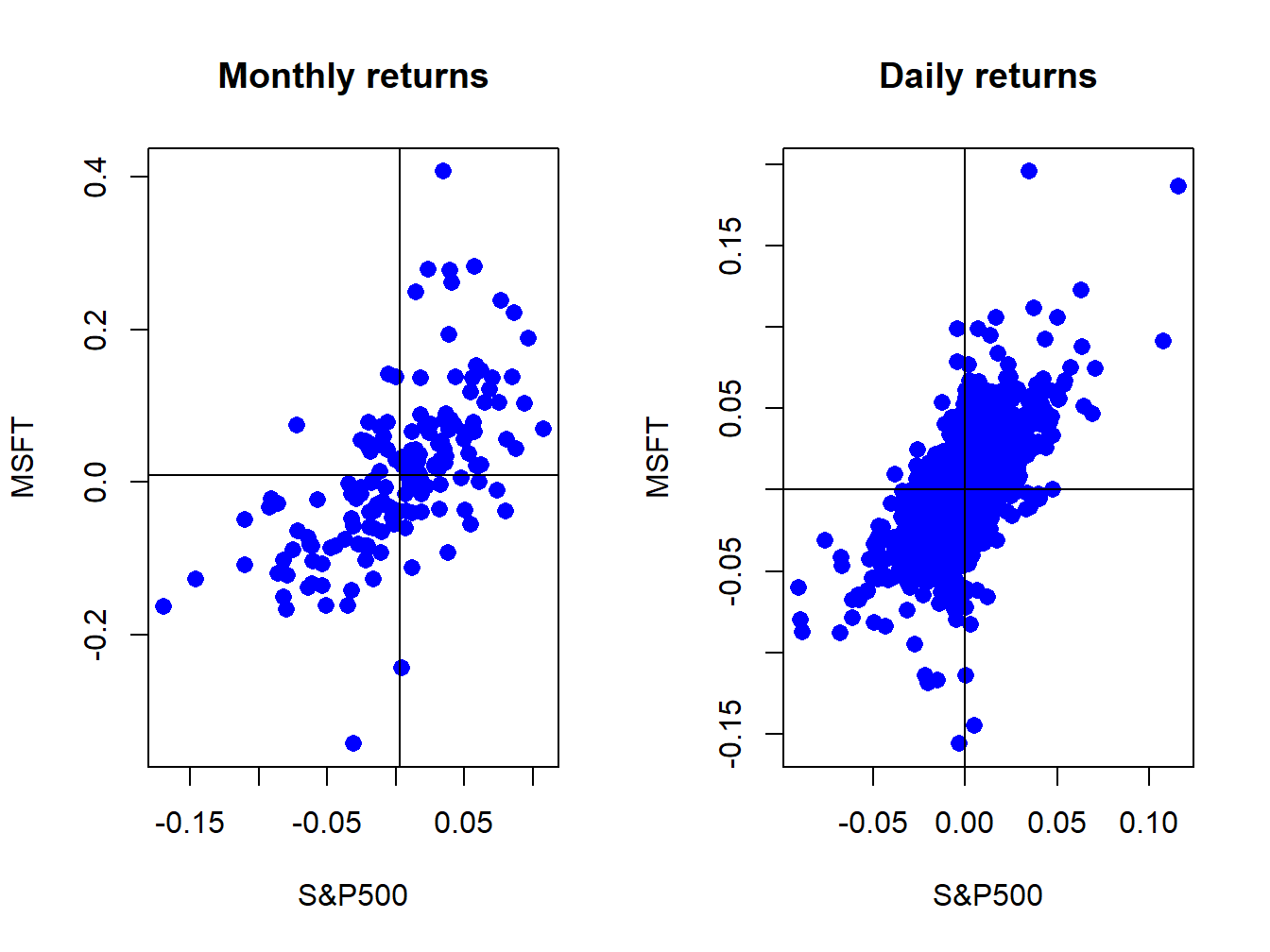
Figure 5.25: Scatterplot of Monthly returns on Microsoft and the S&P 500 index.
The S&P 500 returns are put on the x-axis and the Microsoft returns on the y-axis because the “market”, as proxied by the S&P 500, is often thought as an independent variable driving individual asset returns. The upward sloping orientation of the scatterplots indicate a positive linear dependence between Microsoft and S&P 500 returns at both the monthly and daily frequencies.
\(\blacksquare\)
pairs() plots
all pair-wise scatterplots in a single plot. For example, to plot
all pair-wise scatterplots for the GWN, Microsoft returns and S&P
500 returns use:
dataToPlot = merge(gwnMonthly,msftMonthlyRetS,sp500MonthlyRetS)
pairs(coredata(dataToPlot), col="blue", pch=16, cex=1.25, cex.axis=1.25)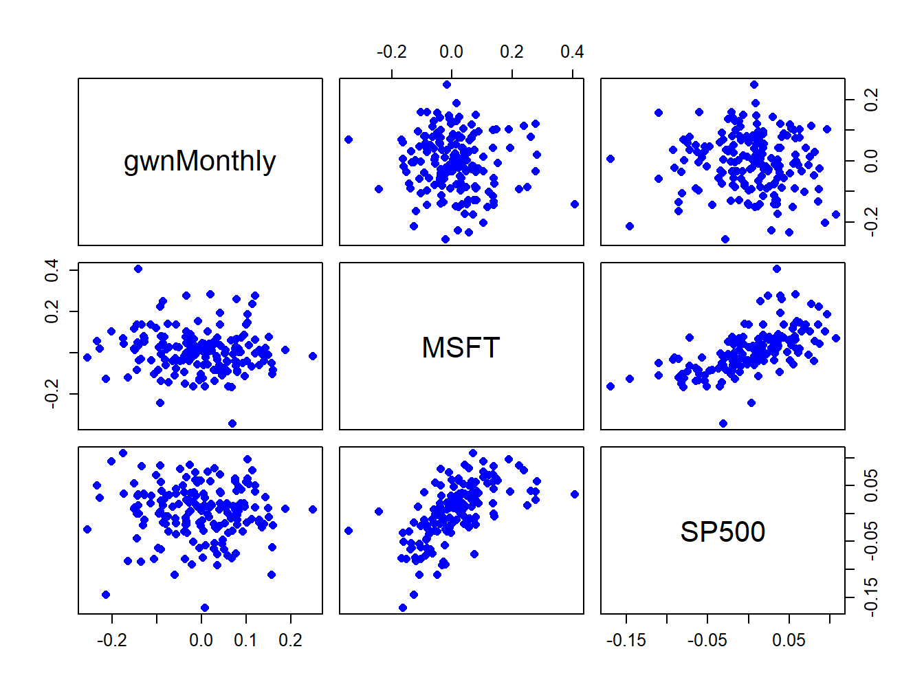
Figure 5.26: Pair-wise scatterplots between simulated GWN, Microsoft returns and S&P 500 returns.
The top row of Figure 5.26 shows the scatterplots between the pairs (MSFT, GWN) and (SP500, GWN), the second row shows the scatterplots between the pairs (GWN, MSFT) and (SP500, MSFT), the third row shows the scatterplots between the pairs (GWN, SP500) and (MSFT, SP500). The plots in the lower triangle are the same as the plots in the upper triangle except the axes are reversed.
\(\blacksquare\)
5.3.2 Sample covariance and correlation
For two random variables \(X\) and \(Y,\) the direction of linear dependence is captured by the covariance, \(\sigma_{XY}=E[(X-\mu_{X})(Y-\mu_{Y})],\) and the direction and strength of linear dependence is captured by the correlation, \(\rho_{XY}=\sigma_{XY}/\sigma_{X}\sigma_{Y}.\) For two data series \(\{x_{t}\}_{t=1}^{T}\) and \(\{y_{t}\}_{t=1}^{T},\) the sample covariance, \[\begin{equation} \hat{\sigma}_{xy}=\frac{1}{T-1}\sum_{t=1}^{T}(x_{t}-\bar{x})(y_{t}-\bar{y}),\tag{5.9} \end{equation}\] measures the direction of linear dependence, and the sample correlation, \[\begin{equation} \hat{\rho}_{xy}=\frac{\hat{\sigma}_{xy}}{\hat{\sigma}_{x}\hat{\sigma}_{x}},\tag{5.10} \end{equation}\] measures the direction and strength of linear dependence. In (5.10), \(\hat{\sigma}_{x}\) and \(\hat{\sigma}_{y}\) are the sample standard deviations of \(\{x_{t}\}_{t=1}^{T}\) and \(\{y_{t}\}_{t=1}^{T},\) respectively, defined by (5.4).
When more than two data series are being analyzed, it is often convenient to compute all pair-wise covariances and correlations at once using matrix algebra. Recall, for a vector of \(N\) random variables \(\mathbf{X}=(X_{1},\ldots,X_{N})^{\prime}\) with mean vector \(\mu=(\mu_{1},\ldots,\mu_{N})^{\prime}\) the \(N\times N\) variance-covariance matrix is defined as: \[ \Sigma=\mathrm{var}(\mathbf{X})=\mathrm{cov}(\mathbf{X})=E[(\mathbf{X}-\mu)(\mathbf{X}-\mu)^{\prime}]=\left(\begin{array}{cccc} \sigma_{1}^{2} & \sigma_{12} & \cdots & \sigma_{1N}\\ \sigma_{12} & \sigma_{2}^{2} & \cdots & \sigma_{2N}\\ \vdots & \vdots & \ddots & \vdots\\ \sigma_{1N} & \sigma_{2N} & \cdots & \sigma_{N}^{2} \end{array}\right). \] For \(N\) data series \(\{x_{t}\}_{t=1}^{T},\) where \(x_{t}=(x_{1t},\ldots,x_{Nt})^{\prime},\) the sample covariance matrix is computed using: \[\begin{equation} \hat{\Sigma}=\frac{1}{T-1}\sum_{t=1}^{T}(\mathbf{x}_{t}-\hat{\mu})(\mathbf{x}_{t}-\hat{\mu})^{\prime}=\left(\begin{array}{cccc} \hat{\sigma}_{1}^{2} & \hat{\sigma}_{12} & \cdots & \hat{\sigma}_{1N}\\ \hat{\sigma}_{12} & \hat{\sigma}_{2}^{2} & \cdots & \hat{\sigma}_{2N}\\ \vdots & \vdots & \ddots & \vdots\\ \hat{\sigma}_{1N} & \hat{\sigma}_{2N} & \cdots & \hat{\sigma}_{N}^{2} \end{array}\right),\tag{5.11} \end{equation}\] where \(\hat{\mu}\) is the \(N\times1\) sample mean vector. Define the \(N\times N\) diagonal matrix: \[\begin{equation} \mathbf{\hat{D}}=\left(\begin{array}{cccc} \hat{\sigma}_{1} & 0 & \cdots & 0\\ 0 & \hat{\sigma}_{2} & \cdots & 0\\ \vdots & \vdots & \ddots & \vdots\\ 0 & 0 & \cdots & \hat{\sigma}_{N} \end{array}\right).\tag{5.12} \end{equation}\] Then the \(N\times N\) sample correlation matrix \(\mathbf{\hat{C}}\) is computed as: \[\begin{equation} \mathbf{\hat{C}}=\mathbf{\hat{D}}^{-1}\hat{\Sigma}\mathbf{\hat{D}}^{-1}=\left(\begin{array}{cccc} 1 & \hat{\rho}_{12} & \cdots & \hat{\rho}_{1N}\\ \hat{\rho}_{12} & 1 & \cdots & \hat{\rho}_{2N}\\ \vdots & \vdots & \ddots & \vdots\\ \hat{\rho}_{1N} & \hat{\rho}_{2N} & \cdots & 1 \end{array}\right).\tag{5.13} \end{equation}\]
The scatterplots of Microsoft and S&P 500 returns in Figure 5.25
suggest positive linear relationships in the data. We can confirm
this by computing the sample covariance and correlation using the
R functions cov() and cor(). For the monthly returns,
we have
##          MSFT
## SP500 0.00298## MSFT
## SP500 0.614Indeed, the sample covariance is positive and the sample correlation shows a moderately strong linear relationship. For the daily returns we have
##           MSFT
## SP500 0.000196## MSFT
## SP500 0.671Here, the daily sample covariance is about twenty times smaller than the monthly covariance (recall the square-root-of time rule), but the daily sample correlation is similar to the monthly sample correlation.
When passed a matrix of data, the cov() and cor()
functions can also be used to compute the sample covariance and correlation
matrices \(\hat{\Sigma}\) and \(\mathbf{\hat{C}}\), respectively.
For example,
##          MSFT   SP500
## MSFT  0.01030 0.00298
## SP500 0.00298 0.00228## MSFT SP500
## MSFT 1.000 0.614
## SP500 0.614 1.000The function cov2cor() transforms a sample covariance matrix
to a sample correlation matrix using (5.13):
##        MSFT SP500
## MSFT  1.000 0.614
## SP500 0.614 1.000\(\blacksquare\)
The R package corrplot contains functions for visualizing
correlation matrices. This is particularly useful for summarizing
the linear dependencies among many data series. For example, Figure
5.27 shows the correlation plot from the corrplot
function corrplot.mixed() created using:
dataToPlot = merge(gwnMonthly, msftMonthlyRetS, sp500MonthlyRetS)
cor.mat = cor(dataToPlot)
corrplot.mixed(cor.mat, lower="number", upper="ellipse")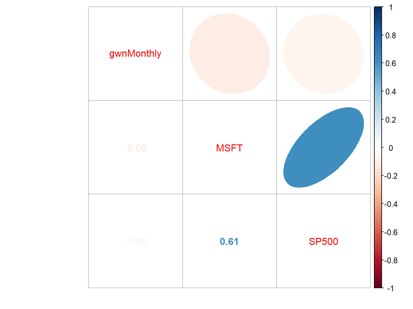
Figure 5.27: Correlation plot created with corrplot().
The color scheme shows the magnitudes of the correlations (blue for positive and red for negative) and the orientation of the ellipses show the magnitude and direction of the linear associations.
\(\blacksquare\)
5.3.3 Sample cross-lag covariances and correlations
The dynamic interactions between two observed time series \(\{x_{t}\}_{t=1}^{T}\)and \(\{y_{t}\}_{t=1}^{T}\) can be measured using the sample cross-lag covariances and correlations
\[\begin{align*} \hat{\gamma}_{xy}^{k} & =\widehat{cov}(X_{t},Y_{t-k}),\\ \hat{\rho}_{xy}^{k} & =\widehat{corr}(X_{t},Y_{t-k})=\frac{\hat{\gamma}_{xy}^{k}}{\sqrt{\hat{\sigma}_{x}^{2}\hat{\sigma}_{y}^{2}}}. \end{align*}\] When more than two data series are being analyzed, all pairwise cross-lag sample covariances and sample correlations can be computed at once using matrix algebra. For a time series of \(N\) data series \(\{\mathbf{x}_{t}\}_{t=1}^{T},\) where \(\mathbf{x}_{t}=(x_{1t},\ldots,x_{Nt})^{\prime},\) the sample lag \(k\) cross-lag covariance and correlation matrices are computed using: \[\begin{eqnarray} \hat{\Gamma}_{k} & = & \frac{1}{T-1}\sum_{t=k+1}^{T}(\mathbf{x}_{t}-\hat{\mu})(\mathbf{x}_{t-k}-\hat{\mu})^{\prime},\tag{5.14}\\ \hat{\mathbf{C}}_{k} & = & \hat{\mathbf{D}}^{-1}\hat{\Gamma}_{k}\hat{\mathbf{D}}^{-1},\tag{5.15} \end{eqnarray}\] where \(\hat{\mathbf{D}}\) is defined in (5.12).
Consider computing the cross-lag covariance and correlation matrices
(5.14) and (5.15) for \(k=0,1,\ldots,5\)
between Microsoft and S&P 500 monthly returns. These matrices may
be computed using the R function acf() as follows:
Ghat = acf(coredata(msftSp500MonthlyRetS), type="covariance",
           lag.max=5, plot=FALSE)
Chat = acf(coredata(msftSp500MonthlyRetS), type="correlation",
           lag.max=5, plot=FALSE)
names(Ghat)
## [1] "acf" "type" "n.used" "lag" "series" "snames"Here, Ghat and Chat are objects of class "acf"
for which there are print and plot methods. The acf components
of Ghat and Chat are 3-dimensional arrays containing
the cross lag matrices (5.14) and (5.15),
respectively. For example, to extract \(\hat{\mathbf{C}}_{0}\) and
\(\hat{\mathbf{C}}_{1}\) use:
##       [,1]  [,2]
## [1,] 1.000 0.614
## [2,] 0.614 1.000## [,1] [,2]
## [1,] -0.1931 -0.0135
## [2,] -0.0307 0.1232The print method shows the sample autocorrelations of each variable as well as the pairwise cross-lag correlations:
##
## Autocorrelations of series 'coredata(msftSp500MonthlyRetS)', by lag
##
## , , MSFT
##
##  MSFT        SP500
##   1.000 ( 0)  0.614 ( 0)
##  -0.193 ( 1) -0.031 (-1)
##  -0.114 ( 2) -0.070 (-2)
##   0.193 ( 3)  0.137 (-3)
##  -0.139 ( 4) -0.030 (-4)
##  -0.023 ( 5)  0.032 (-5)
##
## , , SP500
##
##  MSFT        SP500
##   0.614 ( 0)  1.000 ( 0)
##  -0.014 ( 1)  0.123 ( 1)
##  -0.043 ( 2) -0.074 ( 2)
##   0.112 ( 3)  0.101 ( 3)
##  -0.105 ( 4)  0.073 ( 4)
##  -0.055 ( 5) -0.010 ( 5)
These values can also be visualized using the plot method:
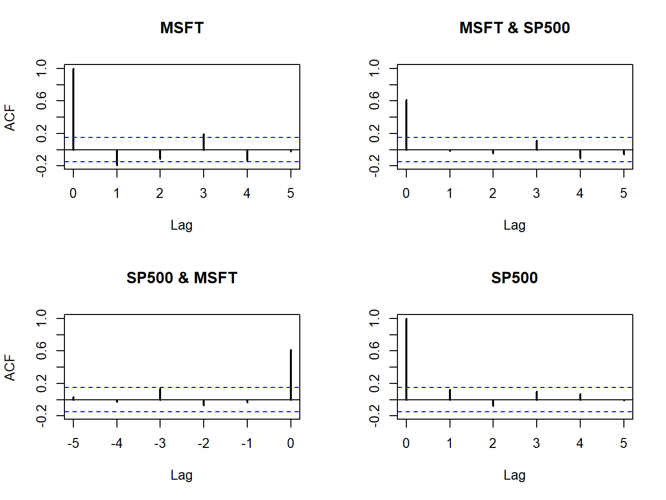
Figure 5.28: Sample cross-lag correlations between Microsoft and S&P 500 returns.
Figure 5.28 shows the resulting four-panel plot. The top-left and bottom-right (diagonal) panels give the SACFs for Microsoft and S&P 500 returns. The top-right plot gives the cross-lag correlations \(\hat{\rho}_{msft,sp500}^{k}\) for \(k=0,1,\ldots,5\) and the bottom-left panel gives the cross-lag correlations \(\hat{\rho}_{sp500,msft}^{k}\) for \(k=0,1,\ldots,5\). The plots show no evidence of any dynamic feedback between the return series.
\(\blacksquare\)