11.4 Efficient portfolios with a risk-free asset
In the preceding section we constructed the efficient set of portfolios involving two risky assets. Now we consider what happens when we introduce a risk-free asset. In the present context, a risk-free asset is equivalent to a default-free pure discount bond that matures at the end of the assumed investment horizon.69 The risk-free rate, \(r_{f}\), is then the nominal return on the bond. For example, if the investment horizon is one month then the risk-free asset is a 30-day U.S. Treasury bill (T-bill) and the risk-free rate is the nominal rate of return on the T-bill.70 If our holdings of the risk-free asset is positive then we are “lending money” to the government at the risk-free rate, and if our holdings are negative then we are “borrowing” from the government at the risk-free rate.
The assumption that investors can borrow and lend at the same risk-free rate is unrealistic in the real world due to differing credit worthiness of investors. Investors can certainly buy T-Bills and receive the risk-free rate. However, most investors can only borrow funds at rates much higher than the T-Bill rate.
11.4.1 Portfolios with one risky asset and one risk-free asset
In this sub-section, we consider portfolios of a single risky asset with random return \(R \sim N(\mu, \sigma^2)\) and a risk-free asset with non-random return \(r_{f}\). Since the risk-free rate is fixed over the investment horizon it is not a random variable. As a result, it has some special properties summarized in the following Proposition.
Proposition 11.2 Let \(r_{f}\) denote the fixed non-random risk-free rate, and let \(R\) denote the random return on a risky asset with \(E[R]=\mu\) and \(\mathrm{var}(R)=\sigma^{2}\). Then \[\begin{align*} E[r_{f}] &= r_{f},\\ \mathrm{var}(r_{f}) & = E[(r_{r}-E[r_{f}])^2] = 0,\\ \mathrm{cov}(R,r_{f}) &= E[(r_{f}-E[r_{f}])(R - E[R])] =0. \end{align*}\]
Consider an investment in the risky asset and the risk-free asset (henceforth referred to as a T-bill). Let \(x\) denote the share of wealth in the risky asset, and \(x_{f}\) denote the share of wealth in T-bills such that \(x + x_{f}=1\). Using \(x_f = 1 - x\), the portfolio return can we written as: \[ R_{p}=x_{f}r_{f}+xR = (1-x)r_{f}+xR=r_{f}+x(R-r_{f}). \tag{11.11} \] The quantity \(R-r_{f}\) is called the excess return (over the return on T-bills) on the risky asset. The portfolio expected return is then:
\[\begin{equation} \mu_{p}=r_{f}+x(E[R]-r_{f})=r_{f}+x(\mu-r_{f}),\tag{11.12} \end{equation}\]
where the quantity \((\mu-r_{f})\) is called the expected excess return or risk premium on the risky asset. The risk premium is typically positive indicating that investors expect a higher return on the risky asset than the safe asset (otherwise, why would investors hold the risky asset?). We may express the risk premium on the portfolio in terms of the risk premium on the risky asset: \[ \mu_{p}-r_{f}=x(\mu-r_{f}). \] The more we invest in the risky asset the higher the risk premium on the portfolio of T-Bills and the risky asset.
Because the risk-free rate is constant, the portfolio variance only depends on the variability of the risky asset and is given by: \[ \sigma_{p}^{2}= \mathrm{var(R_{p})} = \mathrm{var(xR)}= x^{2}\sigma^{2}. \] The portfolio standard deviation is therefore proportional to the standard deviation on the risky asset:71
\[\begin{equation} \sigma_{p}=|x|\sigma.\tag{11.13} \end{equation}\]
To illustrate the risk-return properties of portfolios of a T-Bill and a single risky asset, consider forming portfolios of T-Bills and asset B. Let \(x_{B}\) and \(1-x_{B}\) denote the shares of wealth in asset B and T-Bills, respectively. Assume the T-Bill rate is \(r_f = 0.03\). Then the risk premium on asset B is \(\mu_{B}-r_{r} = 0.055 - 0.03 = 0.025\), the expected return on portfolios of T-Bills and asset B is \(\mu_{p} = 0.03 + x_{B}\times 0.025\), and the portfolio standard deviation is \(\sigma_{p} = |x_{B}|\times 0.115\). Figure 11.6 plots \(\mu_{p}\) vs. \(\sigma_{p}\) for portfolios with \(x_{B} = -1.4, -1.3, \ldots 1.4\).
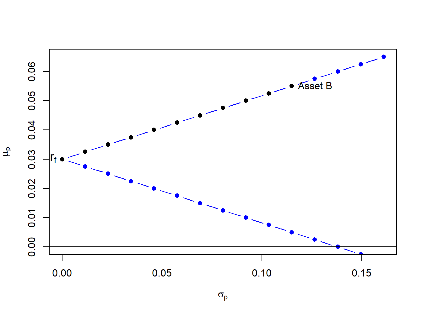
Figure 11.6: Portfolios of T-Bills and asset B for example data.
Notice that the set of feasible portfolios lie on two straight lines, one with a positive slope and one with a negative slope. The line with a positive slope represents portfolios with long positions in asset B, and the line with a negative slope represents portfolios with short positions in asset B. The blue dots represent portfolios with short positions and the black dots represent long-only portfolios. The blue dots above the point labeled “Asset B” represent long-short portfolios where the T-Bill is shorted to finance additional investment in asset B.
\(\blacksquare\)
If we assume that \(x > 0\) (do not short the risky asset), we can use (11.13) to solve for \(x\): \[ x=\frac{\sigma_{p}}{\sigma}. \tag{11.14} \] Substituting (11.14) into (11.12) gives the following equation:
\[\begin{equation} \mu_{p}=r_{f}+\frac{\mu-r_{f}}{\sigma}\cdot\sigma_{p},\tag{11.15} \end{equation}\]
Equation (11.15) describes a straight line in (\(\mu_{p},\sigma_{p}\))-space with intercept \(r_{f}\) and slope \((\mu-r_{f})/\sigma\). This line characterizes the linear risk-return tradeoff of portfolios of T-Bills and a risky asset when the risky asset is not shorted. This line has a positive slope provided the risk premium is positive.
This line described by (11.15) is often called the capital allocation line (CAL) as it describes how investment capital is allocated between T-Bills and the risky asset. Points on the line close to the y-axis represent portfolios mostly allocated to T-Bills, and points far away from the y-axis represent portfolios mostly allocated to the risky asset. The slope of the CAL is called the Sharpe ratio (SR) (named after the economist William Sharpe), and it measures the risk premium on the asset per unit of risk (as measured by the standard deviation of the asset). From (11.15) we have \[ \frac{d\mu_{p}}{d\sigma_{p}}=\frac{\mu-r_{f}}{\sigma}=SR. \]
Consider creating portfolios of asset A and T-bills and asset B and T-Bills with \(r_{f}=0.03\):
r.f = 0.03
x.A = seq(from=0, to=1.4, by=0.1)
mu.p.A = r.f + x.A*(mu.A - r.f)
sig.p.A = x.A*sig.A
x.B = seq(from=0, to=1.4, by=0.1)
mu.p.B = r.f + x.B*(mu.B - r.f)
sig.p.B = x.B*sig.B
The risk-return properties of these portfolios are illustrated in Figure 11.7.
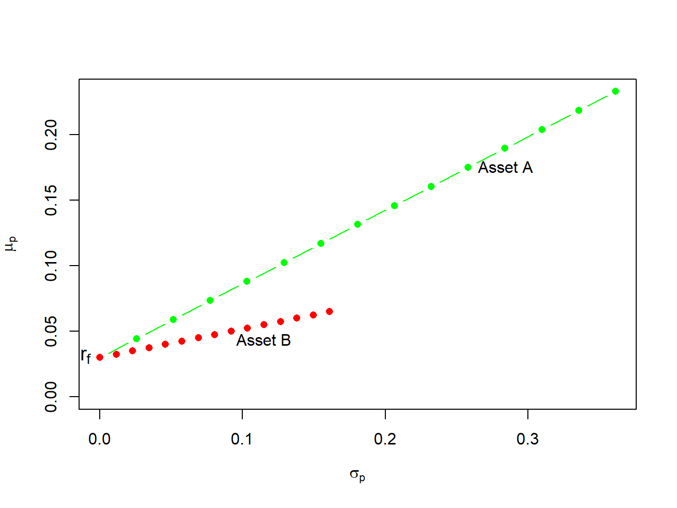
Figure 11.7: Portfolios of T-Bills and risky assets.
In Figure 11.7 the point labeled “\(r_{f}\)” represents a portfolio that is 100% invested in T-bills. The points labeled “Asset A” and “Asset B” represent portfolios that are 100% invested in assets A and B, respectively. A point half-way between “\(r_{f}\)” and “Asset A” is a portfolio that is 50% invested in T-bills and 50% invested in asset A. A point above and to the right of “Asset A” is a levered portfolio where more than 100% of asset A is financed by borrowing at the T-bill rate. Notice that as leverage increases (i.e, borrowing more at the T-Bill rate), portfolio volatility increases.
The portfolios which are combinations of asset A and T-bills have expected returns uniformly higher than the portfolios consisting of asset B and T-bills. This occurs because the Sharpe ratio for asset \(A\) is higher than the ratio for asset \(B\):
\[\begin{align*} \mathrm{SR}_{A} & =\frac{\mu_{A}-r_{f}}{\sigma_{A}}=\frac{0.175-0.03}{0.258}=0.562,\\ \mathrm{SR}_{B} & =\frac{\mu_{B}-r_{f}}{\sigma_{B}}=\frac{0.055-0.03}{0.115}=0.217. \end{align*}\] Hence, portfolios of asset \(A\) and T-bills are efficient relative to portfolios of asset \(B\) and T-bills.
\(\blacksquare\)
The previous example shows that the Sharpe ratio can be used to rank the risk return properties of individual assets. Assets with a high Sharpe ratio have a better risk-return tradeoff than assets with a low Sharpe ratio. Accordingly, investment analysts routinely rank assets based on their Sharpe ratios.
11.4.2 Portfolios with one risky asset and one risk-free asset with different borrowing and lending rates
TBD
In the finance industry the risk-free asset is often referred to as “cash”. In general, “cash” doesn’t refer to holding dollars in your pocket but rather investing dollars in a very low risk asset that pays a stable rate of return.↩︎
The default-free assumption of U.S. debt is often taken for granted. However, this assumption has been questioned due to the inability of the U.S. congress to address the long-term debt problems of the U.S. government.↩︎
Here, we can allow \(x\) to be positive or negative but \(\sigma\) is always positive. ↩︎