4.1 Stochastic Processes

A discrete-time stochastic process or time series process $$\{\ldots,Y_{1},Y_{2},\ldots,Y_{t},Y_{t+1},\ldots\}=\{Y_{t}\}_{t=-\infty}^{\infty},$$ is a sequence of random variables indexed by time $t$¹⁷. In most applications, the time index is a regularly spaced index representing calendar time (e.g., days, months, years, etc.) but it can also be irregularly spaced representing event time (e.g., intra-day transaction times). In modeling time series data, the ordering imposed by the time index is important because we often would like to capture the temporal relationships, if any, between the random variables in the stochastic process. In random sampling from a population, the ordering of the random variables representing the sample does not matter because they are independent.

A realization of a stochastic process with $T$ observations is the sequence of observed data $$\{Y_{1}=y_{1},Y_{2}=y_{2},\ldots,Y_{T}=y_{T}\}=\{y_{t}\}_{t=1}^{T}.$$ The goal of time series modeling is to describe the probabilistic behavior of the underlying stochastic process that is believed to have generated the observed data in a concise way. In addition, we want to be able to use the observed sample to estimate important characteristics of a time series model such as measures of time dependence. In order to do this, we need to make a number of assumptions regarding the joint behavior of the random variables in the stochastic process such that we may treat the stochastic process in much the same way as we treat a random sample from a given population.

4.1.1 Stationary stochastic processes

We often describe random sampling from a population as a sequence of independent, and identically distributed (iid) random variables $X_{1},X_{2}\ldots$ such that each $X_{i}$ is described by the same probability distribution $F_{X}$, and write $X_{i}\sim F_{X}$. With a time series process, we would like to preserve the identical distribution assumption but we do not want to impose the restriction that each random variable in the sequence is independent of all of the other variables. In many contexts, we would expect some dependence between random variables close together in time (e.g, $X_{1}$, and $X_{2})$ but little or no dependence between random variables far apart in time (e.g., $X_{1}$ and $X_{100})$. We can allow for this type of behavior using the concepts of stationarity and ergodicity.

We start with the definition of strict stationarity.

Definition 2.1 (Strict stationarity)

A stochastic process $\{Y_{t}\}$ is strictly stationary if, for any given finite integer $r$ and for any set of subscripts $t_{1},t_{2},\ldots,t_{r}$ the joint distribution of $(Y_{t_{1}},Y_{t_{2}},\ldots,Y_{t_{r}})$ depends only on $t_{1}-t,t_{2}-t,\ldots,t_{r}-t$ but not on $t$. In other words, the joint distribution of $(Y_{t_{1}},Y_{t_{2}},\ldots,Y_{t_{r}})$ is the same as the joint distribution of $(Y_{t_{1}-t},Y_{t_{2}-t},\ldots,Y_{t_{r}-t})$ for any value of $t$.

In simple terms, the joint distribution of random variables in a strictly stationary stochastic process is time invariant. For example, the joint distribution of $(Y_{1},Y_{5},Y_{7})$ is the same as the distribution of $(Y_{12},Y_{16},Y_{18})$. Just like in an iid sample, in a strictly stationary process all of the individual random variables $Y_{t}$ ($t=-\infty,\ldots,\infty$) have the same marginal distribution $F_{Y}$. This means they all have the same mean, variance etc., assuming these quantities exist. However, assuming strict stationarity does not make any assumption about the correlations between $Y_{t},Y_{t_{1}},\ldots,Y_{t_{r}}$ other than that the correlation between $Y_{t}$ and $Y_{t_{r}}$ only depends on $t-t_{r}$ (the time between $Y_{t}$ and $Y_{t_{r}})$ and not on $t$. That is, strict stationarity allows for general temporal dependence between the random variables in the stochastic process.

A useful property of strict stationarity is that it is preserved under general transformations, as summarized in the following proposition.

Proposition 4.1 Let $\{Y_{t}\}$ be strictly stationary and let $g(\cdot)$ be any function of the elements in $\{Y_{t}\}$. Then $\{g(Y_{t})\}$, is also strictly stationary.

For example, if $\{Y_{t}\}$ is strictly stationary then $\{Y_{t}^{2}\}$ and $\{Y_{t}Y_{t-1}\}$ are also strictly stationary.

The following are some simple examples of strictly stationary processes.

Example 4.1 (iid sequence)

If $\{Y_{t}\}$ is an iid sequence, then it is strictly stationary.

$\blacksquare$

Example 4.2 (Non iid sequence)

Let $\{Y_{t}\}$ be an iid sequence and let $X\sim N(0,1)$ independent of $\{Y_{t}\}$. Define $Z_{t}=Y_{t}+X$. The sequence $\{Z_{t}\}$ is not an independent sequence (because of the common $X)$ but is an identically distributed sequence and is strictly stationary.

$\blacksquare$

Strict stationarity places very strong restrictions on the behavior of a time series. A related concept that imposes weaker restrictions and is convenient for time series model building is covariance stationarity (sometimes called weak stationarity).

Definition 4.1 (Covariance stationarity)

A stochastic process $\{Y_{t}\}$ is covariance stationary if

1. $E[Y_{t}]=\mu < \infty$ does not depend on $t$
2. $\mathrm{var}(Y_{t})=\sigma^{2}<\infty$ does not depend on $t$
3. $\mathrm{cov}(Y_{t},Y_{t-j})=\gamma_{j}<\infty$, and depends only on $j$ but not on $t$ for $j=0,1,2,\ldots$

The term $\gamma_{j}$ is called the $j^{\textrm{th}}$ order autocovariance. The $j^{\textrm{th}}$ order autocorrelation is defined as: $$\begin{equation} \rho_{j}=\frac{\mathrm{cov}(Y_{t},Y_{t-j})}{\sqrt{\mathrm{var}(Y_{t})\mathrm{var}(Y_{t-j})}}=\frac{\gamma_{j}}{\sigma^{2}}.\tag{4.1} \end{equation}$$

The autocovariances, $\gamma_{j},$ measure the direction of linear dependence between $Y_{t}$ and $Y_{t-j}$. The autocorrelations, $\rho_{j}$, measure both the direction and strength of linear dependence between $Y_{t}$ and $Y_{t-j}$. With covariance stationarity, instead of assuming the entire joint distribution of a collection of random variables is time invariant we make a weaker assumption that only the mean, variance and autocovariances of the random variables are time invariant. A strictly stationary stochastic process $\{Y_{t}\}$ such that $\mu$, $\sigma^{2}$, and $\gamma_{ij}$ exist is a covariance stationary stochastic process. However, a covariance stationary process need not be strictly stationary.

The autocovariances and autocorrelations are measures of the linear temporal dependence in a covariance stationary stochastic process. A graphical summary of this temporal dependence is given by the plot of $\rho_{j}$ against $j$, and is called the autocorrelation function (ACF). Figure 4.1 illustrates an ACF for a hypothetical covariance stationary time series with $\rho_{j}=(0.9)^{j}$ for $j=1,2,\ldots,10$ created with

rho = 0.9 
rhoVec = (rho)^(1:10) 
ts.plot(rhoVec, type="h", lwd=2, col="blue", xlab="Lag j", 
        ylab=expression(rho[j]))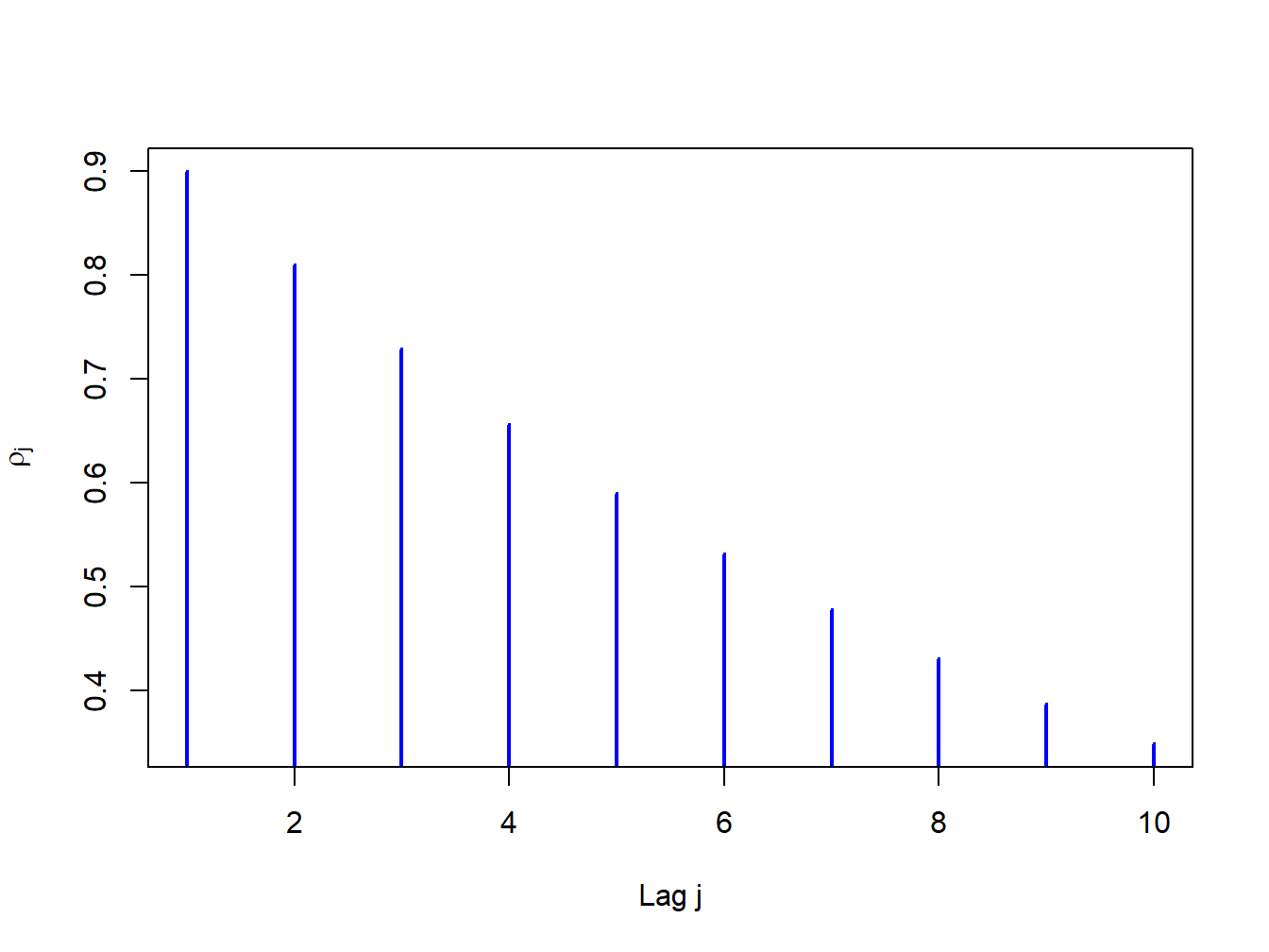

Figure 4.1: ACF for time series with $\rho_{j}=(0.9)^{j}$

For this process the strength of linear time dependence decays toward zero geometrically fast as $j$ increases.

The definition of covariance stationarity requires that $E[Y_{t}]<\infty$ and $\mathrm{var}(Y_{t})<\infty.$ That is, $E[Y_{t}]$ and $\mathrm{var}(Y_{t})$ must exist and be finite numbers. This is true if $Y_{t}$ is normally distributed. However, it is not true if, for example, $Y_{t}$ has a Student’s t distribution with one degree of freedom.¹⁸ Hence, a strictly stationary stochastic process $\{Y_{t}\}$ where the (marginal) pdf of $Y_{t}$ (for all $t$) has very fat tails may not be covariance stationary.

Example 4.3 (Gaussian White Noise)

Let $Y_{t}\sim iid$ $N(0,\sigma^{2})$. Then $\{Y_{t}\}$ is called a Gaussian white noise (GWN) process and is denoted $Y_{t}\sim\mathrm{GWN}(0,\sigma^{2})$. Notice that: $$\begin{align*} E[Y_{t}] & =0\textrm{ independent of }t,\\ \mathrm{var}(Y_{t}) & =\sigma^{2}\textrm{ independent of }t,\\ \mathrm{cov}(Y_{t},Y_{t-j}) & =0\text{ (for }j>0)\text{ independent of }t\textrm{ for all }j, \end{align*}$$ so that $\{Y_{t}\}$ satisfies the properties of a covariance stationary process. The defining characteristic of a GWN process is the lack of any predictable pattern over time in the realized values of the process. The term white noise comes from the electrical engineering literature and represents the absence of any signal.¹⁹

Simulating observations from a GWN process in R is easy: just simulate iid observations from a normal distribution. For example, to simulate $T=250$ observations from the GWN(0,1) process use:

set.seed(123)
y = rnorm(250)

The simulated iid N(0,1) values are generated using the rnorm() function. The command set.seed(123) initializes R’s internal random number generator using the seed value 123. Every time the random number generator seed is set to a particular value, the random number generator produces the same set of random numbers. This allows different people to create the same set of random numbers so that results are reproducible. The simulated data is illustrated in Figure 4.2 created using:

ts.plot(y,main="Gaussian White Noise Process",xlab="time",
        ylab="y(t)", col="blue", lwd=2)
abline(h=0)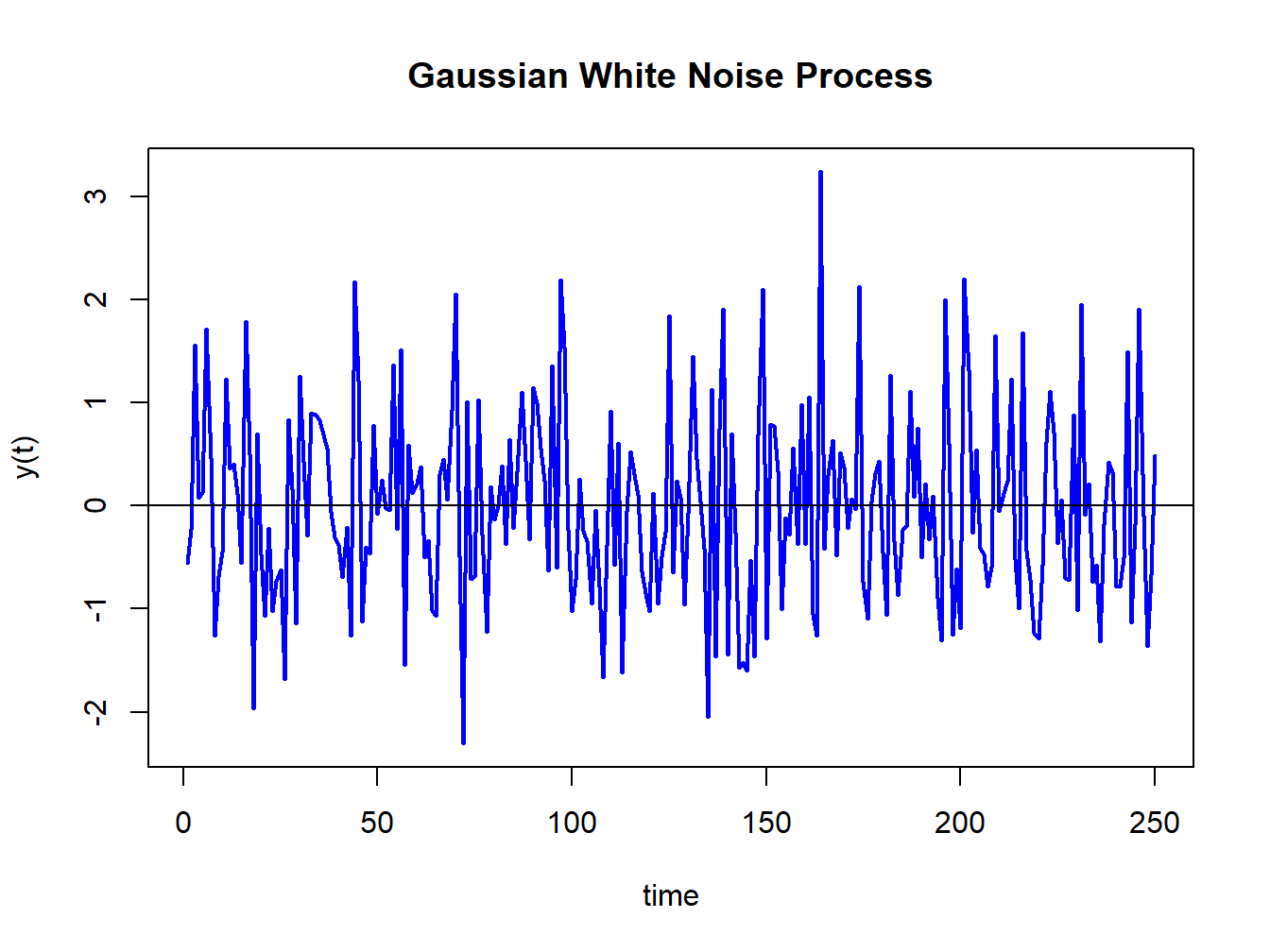

Figure 4.2: Realization of a GWN(0,1) process.

The function ts.plot() creates a time series line plot with a dummy time index. An equivalent plot can be created using the generic plot() function with optional argument type="l". The data in Figure 4.2 fluctuate randomly about the mean value zero and exhibit a constant volatility of one (typical magnitude of a fluctuation about zero). There is no visual evidence of any predictable pattern in the data.

$\blacksquare$

Example 2.5 (GWN model for continuously compounded returns)

Let $r_{t}$ denote the continuously compounded monthly return on Microsoft stock and assume that $r_{t}\sim\mathrm{iid}\,N(0.01,\,(0.05)^{2})$. We can represent this distribution in terms of a GWN process as follows $$r_{t}=0.01+\varepsilon_{t},\,\varepsilon_{t}\sim\mathrm{GWN}(0,\,(0.05)^{2}).$$ Here, $r_{t}$ is constructed as a $\mathrm{GWN}(0,\sigma^{2})$ process plus a constant. Hence, $\{r_{t}\}$ is a GWN process with a non-zero mean: $r_{t}\sim\mathrm{GWN}(0.01,\,(0.05)^{2}).$ $T=60$ simulated values of $\{r_{t}\}$ are computed using:

set.seed(123)
y = rnorm(60, mean=0.01, sd=0.05)
ts.plot(y,main="GWN Process for Monthly Continuously Compounded Returns",
        xlab="time",ylab="r(t)", col="blue", lwd=2)
abline(h=c(0,0.01,-0.04,0.06), lwd=2, 
       lty=c("solid","solid","dotted","dotted"), 
       col=c("black", "red", "red", "red"))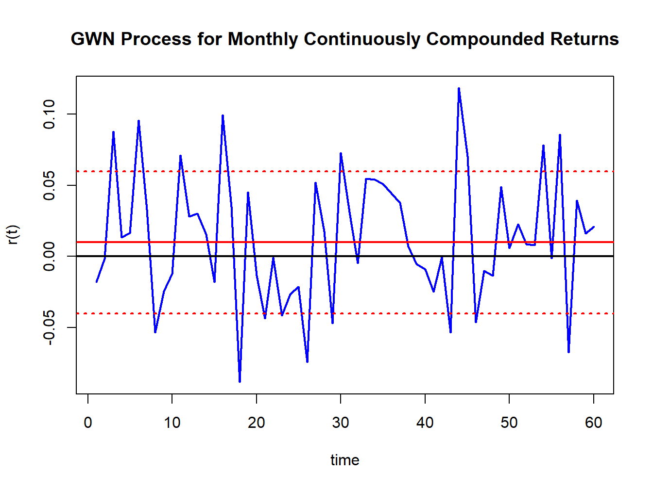

Figure 4.3: Simulated returns from GWN(0.01,(0.05)$^{2})$.

and are illustrated in Figure 4.3. Notice that the returns fluctuate around the mean value of $0.01$ (solid red line) and the size of a typical deviation from the mean is about $0.05$. The red dotted lines show the values $0.1 \pm 0.05$ .

An implication of the GWN assumption for monthly returns is that non-overlapping multi-period returns are also GWN. For example, consider the two-month return $r_{t}(2)=r_{t}+r_{t-1}$. The non-overlapping process $\{r_{t}(2)\}=\{...,r_{t-2}(2),r_{t}(2),r_{t+2}(2),...\}$ is GWN with mean $E[r_{t}(2)]=2\cdot\mu=0.02$, variance $\mathrm{var}(r_{t}(2))=2\cdot\sigma^{2}=0.005$, and standard deviation $\mathrm{sd}(r_{t}(2))=\sqrt{2}\sigma=0.071$.

$\blacksquare$

Example 3.2 (Independent white noise)

Let $Y_{t}\sim\mathrm{iid}$ $(0,\sigma^{2})$. Then $\{Y_{t}\}$ is called an independent white noise (IWN) process and is denoted $Y_{t}\sim\mathrm{IWN}(0,\sigma^{2})$. The difference between GWN and IWN is that with IWN we don’t specify that all random variables are normally distributed. The random variables can have any distribution with mean zero and variance $\sigma^{2}.$ To illustrate, suppose $Y_{t}=\frac{1}{\sqrt{3}}\times t_{3}$ where $t_{3}$ denotes a Student’s t distribution with $3$ degrees of freedom. This process has $E[Y_{t}]=0$ and $\mathrm{var}(Y_{t})=1.$ Figure 4.4 shows simulated observations from this process created using the R commands

set.seed(123) 
y = (1/sqrt(3))*rt(250, df=3) 
ts.plot(y, main="Independent White Noise Process", xlab="time", ylab="y(t)",         
        col="blue", lwd=2) 
abline(h=0)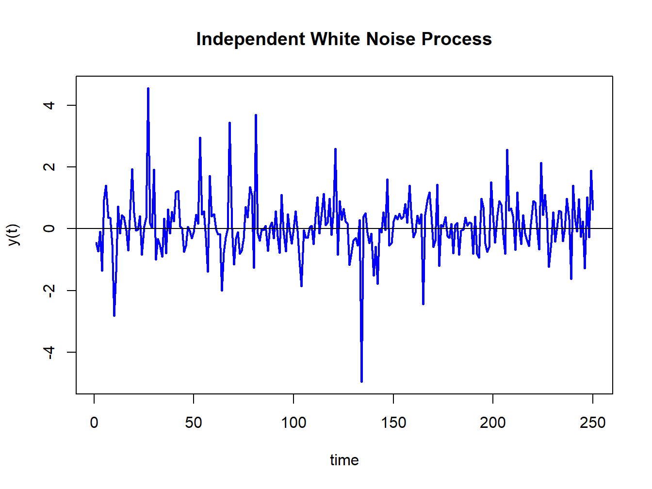

Figure 4.4: Simulation of IWN(0,1) process: $Y_{t}\sim\frac{1}{\sqrt{3}}\times t_{3}$

The simulated IWN process resembles the GWN in Figure 4.4 but has more extreme observations.

$\blacksquare$

Example 2.6 (Weak white noise)

Let $\{Y_{t}\}$ be a sequence of uncorrelated random variables each with mean zero and variance $\sigma^{2}$. Then $\{Y_{t}\}$ is called a weak white noise (WWN) process and is denoted $Y_{t}\sim\mathrm{WWN}(0,\sigma^{2})$. With a WWN process, the random variables are not independent, only uncorrelated. This allows for potential non-linear temporal dependence between the random variables in the process.

$\blacksquare$

4.1.2 Non-Stationary processes

In a covariance stationary stochastic process it is assumed that the means, variances and autocovariances are independent of time. In a non-stationary process, one or more of these assumptions is not true. The following examples illustrate some typical non-stationary time series processes.

Example 2.7 (Deterministically trending process)

Suppose $\{Y_{t}\}$ is generated according to the deterministically trending process: $$\begin{align*} Y_{t} & =\beta_{0}+\beta_{1}t+\varepsilon_{t},~\varepsilon_{t}\sim\mathrm{GWN}(0,\sigma_{\varepsilon}^{2}),\\ t & =0,1,2,\ldots \end{align*}$$ Then $\{Y_{t}\}$ is nonstationary because the mean of $Y_{t}$ depends on $t$: $$E[Y_{t}]=\beta_{0}+\beta_{1}t.$$ Figure 4.5 shows a realization of this process with $\beta_{0}=0,\beta_{1}=0.1$ and $\sigma_{\varepsilon}^{2}=1$ created using the R commands:

set.seed(123)
e = rnorm(250)
y.dt = 0.1*seq(1,250) + e
ts.plot(y.dt, lwd=2, col="blue", main="Deterministic Trend + Noise")
abline(a=0, b=0.1)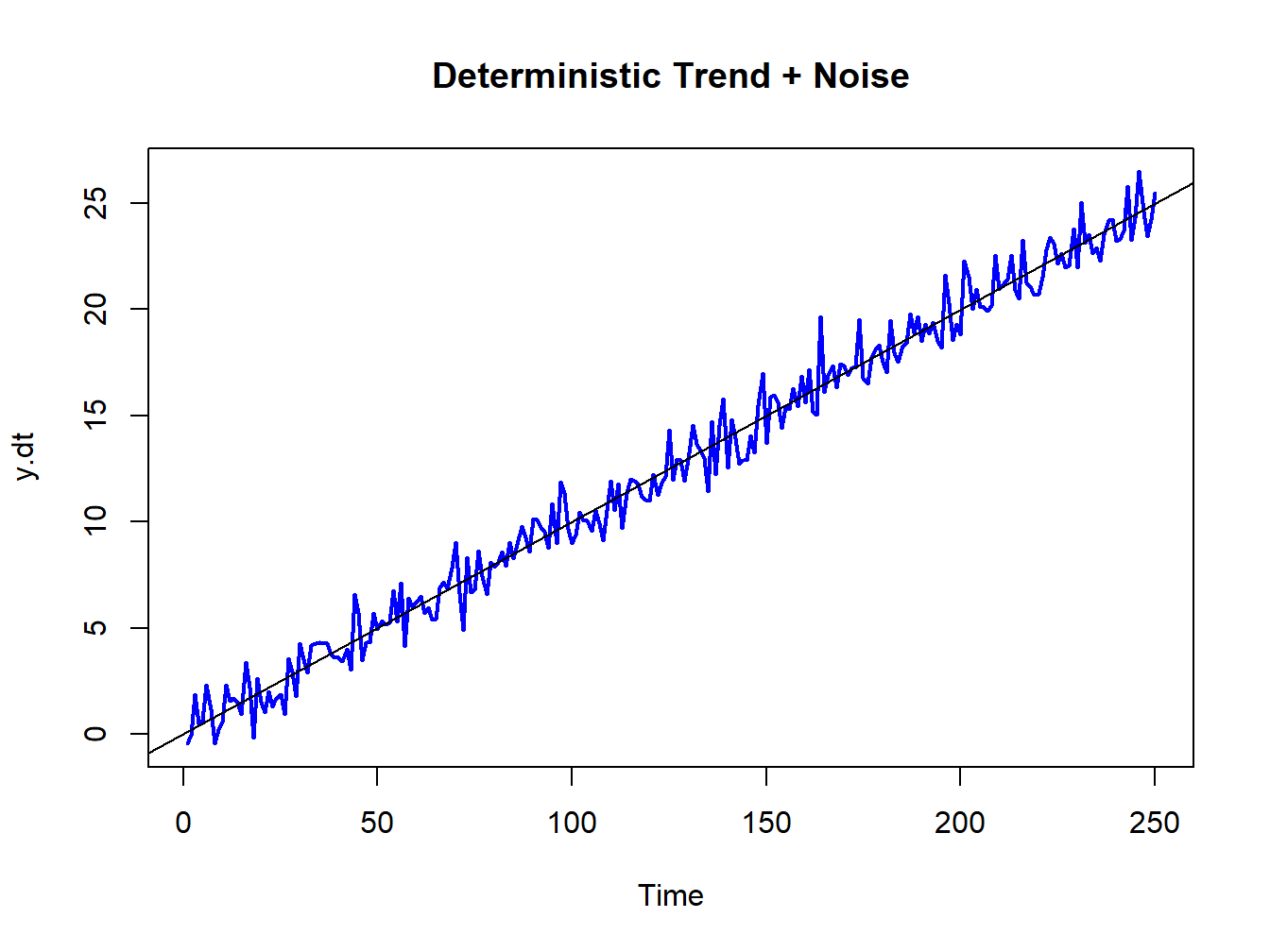

Figure 4.5: Deterministically trending nonstationary process $Y_{t}=0.1\times t+\varepsilon_{t},\varepsilon_{t}\sim\mathrm{GWN}(0,1)$

Here the non-stationarity is created by the deterministic trend $\beta_{0}+\beta_{1}t$ in the data. The non-stationary process $\{Y_{t}\}$ can be transformed into a stationary process by simply subtracting off the trend: $$X_{t}=Y_{t}-\beta_{0}-\beta_{1}t=\varepsilon_{t}\sim\mathrm{GWN}(0,\sigma_{\varepsilon}^{2}).$$ The detrended process $X_{t}\sim\mathrm{GWN}(0,\sigma_{\varepsilon}^{2})$ is obviously covariance stationary.

$\blacksquare$

Example 2.8 (Random walk)

A random walk (RW) process $\{Y_{t}\}$ is defined as: $$\begin{align*} Y_{t} & =Y_{t-1}+\varepsilon_{t},~\varepsilon_{t}\sim\mathrm{GWN}(0,\sigma_{\varepsilon}^{2}),\\ & Y_{0}\textrm{ is fixed (non-random)}. \end{align*}$$ By recursive substitution starting at $t=1$, we have: $$\begin{align*} Y_{1} & =Y_{0}+\varepsilon_{1},\\ Y_{2} & =Y_{1}+\varepsilon_{2}=Y_{0}+\varepsilon_{1}+\varepsilon_{2},\\ & \vdots\\ Y_{t} & =Y_{t-1}+\varepsilon_{t}=Y_{0}+\varepsilon_{1}+\cdots+\varepsilon_{t}\\ & =Y_{0}+\sum_{j=1}^{t}\varepsilon_{j}. \end{align*}$$ Now, $E[Y_{t}]=Y_{0}$ which is independent of $t$. However, $$\mathrm{var}(Y_{t})=\mathrm{var}\left(\sum_{j=1}^{t}\varepsilon_{j}\right)=\sum_{j=1}^{t}\sigma_{\varepsilon}^{2}=\sigma_{\varepsilon}^{2}\times t,$$ which depends on $t$, and so $\{Y_{t}\}$ is not stationary.

Figure 4.6 shows a realization of the RW process with $Y_{0}=0$ and $\sigma_{\varepsilon}^{2}=1$ created using the R commands:

set.seed(321)
e = rnorm(250)
y.rw = cumsum(e)
ts.plot(y.rw, lwd=2, col="blue", main="Random Walk")
abline(h=0)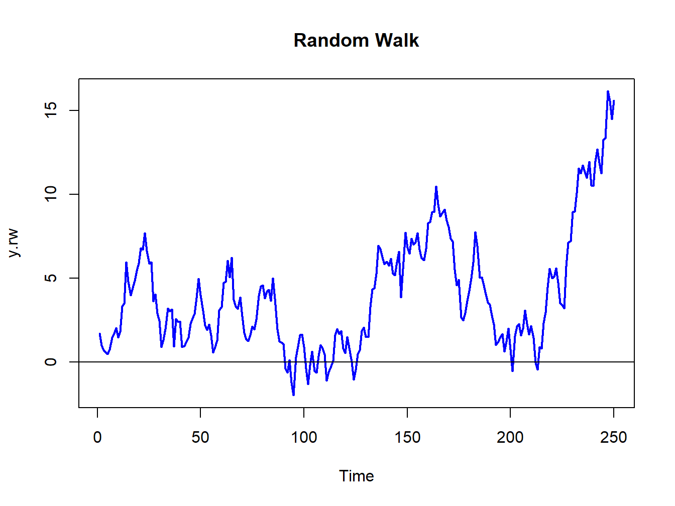

Figure 4.6: Random walk process: $Y_{t}=Y_{t-1}+\varepsilon_{t},\varepsilon_{t}\sim\mathrm{GWN}(0,1)$.

The RW process looks much different from the GWN process in Figure 4.2. As the variance of the process increases linearly with time, the uncertainty about where the process will be at a given point in time increases with time.

Although $\{Y_{t}\}$ is non-stationary, a simple first-differencing transformation, however, yields a covariance stationary process: $$X_{t}=Y_{t}-Y_{t-1}=\varepsilon_{t}\sim\mathrm{GWN}(0,\sigma_{\varepsilon}^{2}).$$

$\blacksquare$

Example 4.4 (Random walk with drift model for log stock prices)

Let $r_{t}$ denote the continuously compounded monthly return on Microsoft stock and assume that $r_{t}\sim\mathrm{GWN}(\mu,\,\sigma^{2})$. Since $r_{t}=\ln(P_{t}/P_{t-1})$ it follows that $\ln P_{t}=\ln P_{t-1}+r_{t}$. Now, re-express $r_{t}$ as $r_{t}=\mu+\varepsilon_{t}$ where $\varepsilon_{t}\sim\mathrm{GWN}(0,\sigma^{2}).$ Then $lnP_{t}=lnP_{t-1}+\mu+\varepsilon_{t}.$ By recursive substitution we have $lnP_{t}=lnP_{0}+\mu t+\sum_{t=1}^{t}\varepsilon_{t}$ and so $\ln P_{t}$ follows a random walk process with drift value $\mu$. Here, $E[lnP_{t}]=\mu t$ and $\mathrm{var}(lnP_{t})=\sigma^{2}t$ so $lnP_{t}$ is non-stationary because both the mean and variance depend on $t$. In this model, prices, however, do not follow a random walk since $P_{t}=e^{\ln P_{t}}=P_{t-1}e^{r_{t}}$.

$\blacksquare$

4.1.3 Ergodicity

In a strictly stationary or covariance stationary stochastic process no assumption is made about the strength of dependence between random variables in the sequence. For example, in a covariance stationary stochastic process it is possible that $\rho_{1}=\mathrm{cor}(Y_{t},Y_{t-1})=\rho_{100}=\mathrm{cor}(Y_{t},Y_{t-100})=0.5$, say. However, in many contexts it is reasonable to assume that the strength of dependence between random variables in a stochastic process diminishes the farther apart they become. That is, $\rho_{1}>\rho_{2}\cdots$ and that eventually $\rho_{j}=0$ for $j$ large enough. This diminishing dependence assumption is captured by the concept of ergodicity.

Definition 4.2 (Ergodicity (intuitive definition))

Intuitively, a stochastic process $\{Y_{t}\}$ is ergodic if any two collections of random variables partitioned far apart in the sequence are essentially independent.

The formal definition of ergodicity is highly technical and requires advanced concepts in probability theory. However, the intuitive definition captures the essence of the concept. The stochastic process $\{Y_{t}\}$ is ergodic if $Y_{t}$ and $Y_{t-j}$ are essentially independent if $j$ is large enough.

If a stochastic process $\{Y_{t}\}$ is covariance stationary and ergodic then strong restrictions are placed on the joint behavior of the elements in the sequence and on the type of temporal dependence allowed.

Example 2.10 (White noise processes)

If $\{Y_{t}\}$ is GWN or IWN then it is both covariance stationary and ergodic.

$\blacksquare$

Example 2.11 (Covariance stationary but not ergodic process (White 1984, page 41))

Let $Y_{t}\sim\mathrm{GWN}(0,1)$ and let $X\sim N(0,1)$ independent of $\{Y_{t}\}$. Define $Z_{t}=Y_{t}+X$. Then $\{Z_{t}\}$ is covariance stationary but not ergodic. To see why $\{Z_{t}\}$ is not ergodic, note that for all $j>0$: $$\begin{align*} \mathrm{var}(Z_{t}) & =\mathrm{var}(Y_{t}+X)=1+1=2,\\ \gamma_{j} & =\mathrm{cov}(Y_{t}+X,Y_{t-j}+X)=\mathrm{cov}(Y_{t},Y_{t-j})+\mathrm{cov}(Y_{t},X)+\mathrm{cov}(Y_{t-j},X)+\mathrm{cov}(X,X)\\ & =\mathrm{cov}(X,X)=\mathrm{var}(X)=1,\\ \rho_{j} & =\frac{1}{2}\text{ for all }j. \end{align*}$$ Hence, the correlation between random variables separated far apart does not eventually go to zero and so $\{Z_{t}\}$ cannot be ergodic.

$\blacksquare$

---

17. To conserve on notation, we will represent the stochastic process $\{Y_{t}\}_{t=-\infty}^{\infty}$ simply as $\{Y_{t}\}.$↩︎

18. This is also called a Cauchy distribution. For this distribution $E[Y_{t}]=\mathrm{var}(Y_{t})=\mathrm{cov}(Y_{t},Y_{t-j})=\infty.$↩︎

19. As an example of white noise, think of tuning an AM radio. In between stations there is no signal and all you hear is static. This is white noise.↩︎