12.4 Computing the Mean-Variance Efficient Frontier
The analytic expression for a minimum variance portfolio (12.21) can be used to show that any minimum variance portfolio can be created as a linear combination of any two minimum variance portfolios with different target expected returns. If the expected return on the resulting portfolio is greater than the expected return on the global minimum variance portfolio, then the portfolio is an efficient frontier portfolio. Otherwise, the portfolio is an inefficient frontier portfolio. As a result, to compute the portfolio frontier in \((\mu_{p},\sigma_{p})\) space (Markowitz bullet) we only need to find two efficient portfolios. The remaining frontier portfolios can then be expressed as linear combinations of these two portfolios. The following proposition describes the process for the three risky asset case using matrix algebra.
Let \(\mathbf{x}\) and \(\mathbf{y}\) be any two minimum variance portfolios with different target expected returns \(\mathbf{x}^{\prime}\mu=\mu_{p,0}\neq\mathbf{y}^{\prime}\mu=\mu_{p,1}\). That is, portfolio \(\mathbf{x}\) solves: \[\begin{align*} \min_{\mathbf{x}}~\sigma_{p,x}^{2}&=\mathbf{x}^{\prime}\Sigma \mathbf{x}\\ \textrm{ s.t. }\mathbf{x}^{\prime}\mu&=\mu_{p,0}\textrm{ and }\mathbf{x}^{\prime}\mathbf{1}=1, \end{align*}\] and portfolio \(\mathbf{y}\) solves, \[\begin{align*} \min_{\mathbf{y}}\sigma_{p,y}^{2}&=\mathbf{y}^{\prime}\Sigma \mathbf{y}\\ \textrm{ s.t. }\mathbf{y}^{\prime}\mu&=\mu_{p,1}\textrm{ and }\mathbf{y}^{\prime}\mathbf{1}=1. \end{align*}\] Let \(\alpha\) be any constant and define the portfolio \(\mathbf{z}\) as a linear combination of portfolios \(\mathbf{x}\) and \(\mathbf{y}\): \[\begin{align} \mathbf{z} & =\alpha\cdot\mathbf{x}+(1-\alpha)\cdot\mathbf{y}\tag{12.22}\\ & =\left(\begin{array}{c} \alpha x_{1}+(1-\alpha)y_{1}\\ \vdots\\ \alpha x_{N}+(1-\alpha)y_{N} \end{array}\right).\nonumber \end{align}\] Then the following results hold:
- The portfolio \(\mathbf{z}\) is a minimum variance portfolio with expected return and variance given by: \[\begin{align} \mu_{p,z} & =\mathbf{z}^{\prime}\mu=\alpha\cdot\mu_{p,x}+(1-\alpha)\cdot\mu_{p,y},\tag{12.23}\\ \sigma_{p,z}^{2} & =\mathbf{z}^{\prime}\mathbf{\Sigma z=\alpha}^{2}\sigma_{p,x}^{2}+(1-\alpha)^{2}\sigma_{p,y}^{2}+2\alpha(1-\alpha)\sigma_{xy},\tag{12.24} \end{align}\] where \(\sigma_{p,x}^{2}=\mathbf{x}^{\prime}\Sigma \mathbf{x},\sigma_{p,y}^{2}=\mathbf{y}^{\prime}\Sigma \mathbf{y},\sigma_{xy}=\mathbf{x}^{\prime}\Sigma \mathbf{y}.\)
- If \(\mu_{p,z}\geq\mu_{p,m}\), where \(\mu_{p,m}\) is the expected return on the global minimum variance portfolio, then portfolio \(\mathbf{z}\) is an efficient frontier portfolio. Otherwise, \(\mathbf{z}\) is an inefficient frontier portfolio.
The proof of 1. follows directly from applying (12.21) to portfolios \(\mathbf{x}\) and \(\mathbf{y}\): \[\begin{align*} \mathbf{x} & =\Sigma^{-1}\mathbf{MB}^{-1}\tilde{\mu}_{x},\\ \mathbf{y} & =\Sigma^{-1}\mathbf{MB}^{-1}\tilde{\mu}_{y}, \end{align*}\] where \(\tilde{\mu}_{x}=(\mu_{p,x},1)^{\prime}\) and \(\tilde{\mu}_{y}=(\mu_{p,y},1)^{\prime}\). Then, for portfolio \(\mathbf{z}\): \[\begin{align*} \mathbf{z} & =\alpha\cdot\mathbf{x}+(1-\alpha)\cdot\mathbf{y}\\ & =\alpha\cdot\Sigma^{-1}\mathbf{MB}^{-1}\tilde{\mu}_{x}+(1-\alpha)\cdot\Sigma^{-1}\mathbf{MB}^{-1}\tilde{\mu}_{y}\\ & =\Sigma^{-1}\mathbf{MB}^{-1}(\alpha\cdot\tilde{\mu}_{x}+(1-\alpha)\cdot\tilde{\mu}_{y})\\ & =\Sigma^{-1}\mathbf{MB}^{-1}\tilde{\mu}_{z}, \end{align*}\] where \(\tilde{\mu}_{z}=\alpha\cdot\tilde{\mu}_{x}+(1-\alpha)\cdot\tilde{\mu}_{y}=(\mu_{p,z},1)^{\prime}\). Result 2. follows from the definition of an efficient portfolio.
Consider the data in Table 1 and the previously computed minimum variance portfolios that have the same expected return as Microsoft and Starbucks, respectively, and let \(\alpha=0.5\). From (12.22), the frontier portfolio \(\mathbf{z}\) is constructed using: \[\begin{align*} \mathbf{z} & =\alpha\cdot\mathbf{x}+(1-\alpha)\cdot\mathbf{y}\\ & =0.5\cdot\left(\begin{array}{c} 0.8275\\ -0.0907\\ 0.2633 \end{array}\right)+0.5\cdot\left(\begin{array}{c} 0.519\\ 0.273\\ 0.207 \end{array}\right)\\ & =\left(\begin{array}{c} (0.5)(0.8275)\\ (0.5)(-0.0907)\\ (0.5)(0.2633) \end{array}\right)+\left(\begin{array}{c} (0.5)(0.519)\\ (0.5)(0.273)\\ (0.5)(0.207) \end{array}\right)\\ & =\left(\begin{array}{c} 0.6734\\ 0.0912\\ 0.2354 \end{array}\right)=\left(\begin{array}{c} z_{A}\\ z_{B}\\ z_{C} \end{array}\right). \end{align*}\] In R, the new frontier portfolio is computed using:
##   MSFT   NORD   SBUX
## 0.6734 0.0912 0.2354
Using \(\mu_{p,z}=\mathbf{z}^{\prime}\mu\) and \(\sigma_{p,z}^{2}=\mathbf{z}^{\prime}\mathbf{\Sigma z}\), the expected return, variance and standard deviation of this portfolio are:
mu.pz = as.numeric(crossprod(z.vec, mu.vec))
sig2.pz = as.numeric(t(z.vec)%*%sigma.mat%*%z.vec)
sig.pz = sqrt(sig2.pz)
c(mu.pz, sig.pz)
## [1] 0.0356 0.0801Equivalently, using \(\mu_{p,z}=\alpha\mu_{p,x}+(1-\alpha)\mu_{p,y}\) and \(\sigma_{p,z}^{2}=\alpha^{2}\sigma_{p,x}^{2}+(1-\alpha)^{2}\sigma_{p,y}^{2}+2\alpha(1-\alpha)\sigma_{xy}\) the expected return, variance and standard deviation of this portfolio are:
mu.pz = a*mu.px + (1-a)*mu.py
sig.xy = as.numeric(t(x.vec)%*%sigma.mat%*%y.vec)
sig2.pz = a^2 * sig2.px + (1-a)^2 * sig2.py + 2*a*(1-a)*sig.xy
sig.pz = sqrt(sig2.pz)
c(mu.pz, sig.pz)
## [1] 0.0356 0.0801Because \(\mu_{p,z}=0.0356>\mu_{p,m}=0.0249\) the frontier portfolio \(\mathbf{z}\) is an efficient frontier portfolio. The three efficient frontier portfolios \(\mathbf{x},\,\mathbf{y}\) and \(\mathbf{z}\) are illustrated in Figure 12.6 and are labeled “E1” , “E2” and “E3” , respectively.
\(\blacksquare\)
Given the two minimum variance portfolios with target expected returns equal to the expected returns on Microsoft and Starbucks, respectively, consider creating a frontier portfolio with target expected return equal to \(0.05\). To determine the value of \(\alpha\) that corresponds with this portfolio we use the equation \[ \mu_{p,z}=\alpha_{.05}\mu_{p,x}+(1-\alpha_{.05})\mu_{p,y}=0.05. \] We can then solve for \(\alpha_{.05}\): \[ \alpha_{.05}=\frac{0.05-\mu_{p,y}}{\mu_{p,x}-\mu_{p,y}}=\frac{0.05-0.0285}{0.0427-0.0285}=1.51. \] Given \(\alpha_{.05}\) we can solve for the portfolio weights using: \[\begin{eqnarray*} \mathbf{z}_{.05} & = & \alpha_{.05}\mathbf{x}+(1-\alpha_{.05})\mathbf{y}\\ & = & 1.51\times\left(\begin{array}{c} 0.8275\\ -0.0907\\ 0.2633 \end{array}\right)-0.514\times\left(\begin{array}{c} 0.519\\ 0.273\\ 0.207 \end{array}\right)\\ & = & \left(\begin{array}{c} 0.986\\ -0.278\\ 0.292 \end{array}\right). \end{eqnarray*}\] We can then compute the mean and variance of this portfolio using \(\mu_{p,z_{.05}}=\mathbf{z}_{.05}^{\prime}\mu\) and \(\sigma_{p,z_{.05}}^{2}=\mathbf{z}_{.05}^{\prime}\mathbf{\Sigma z}_{.05}.\) Using R, the calculations are:
## [1] 1.51## MSFT NORD SBUX
## 0.986 -0.278 0.292# compute mean and volatility
mu.pz.05 = as.numeric(crossprod(z.05,mu.vec))
sig.pz.05 = as.numeric(sqrt(t(z.05)%*%sigma.mat%*%z.05))
c(mu.pz.05,sig.pz.05)## [1] 0.050 0.107This portfolio is labeled “E4” in Figure 12.6.
Given the two minimum variance portfolios with target expected returns equal to the expected returns on Microsoft and Starbucks, respectively, consider creating a frontier portfolio with target expected return equal to the expected return on Nordstrom. Then, \[ \mu_{p,z}=\alpha_{nord}\mu_{p,x}+(1-\alpha_{nord})\mu_{p,y}=\mu_{\textrm{nord}}=0.0015, \] and we can solve for \(\alpha_{nord}\) using: \[ \alpha_{nord}=\frac{\mu_{\textrm{nord}}-\mu_{p,y}}{\mu_{p,x}-\mu_{p,y}}=\frac{0.0015-0.0285}{0.0427-0.0285}=-1.901. \] The portfolio weights are: \[\begin{eqnarray*} \mathbf{z}_{nord} & = & \alpha_{nord}\mathbf{x}+(1-\alpha_{nord})\mathbf{y}\\ & = & -1.901\times\left(\begin{array}{c} 0.8275\\ -0.0907\\ 0.2633 \end{array}\right)+2.9\times\left(\begin{array}{c} 0.519\\ 0.273\\ 0.207 \end{array}\right)\\ & = & \left(\begin{array}{c} -0.0064\\ 0.9651\\ 0.1013 \end{array}\right). \end{eqnarray*}\] Using R, the calculations are:
## NORD
## -1.9## MSFT NORD SBUX
## -0.0664 0.9651 0.1013# compute mean and volatility
mu.pz.nord = as.numeric(crossprod(z.nord,mu.vec))
sig.pz.nord = as.numeric(sqrt(t(z.nord)%*%sigma.mat%*%z.nord))
c(mu.pz.nord,sig.pz.nord)## [1] 0.0015 0.1033Because \(\mu_{p,z}=0.0015<\mu_{p,m}=0.02489\) the frontier portfolio \(\mathbf{z}\) is an inefficient frontier portfolio. This portfolio is labeled “IE1” in Figure 12.6.
\(\blacksquare\)
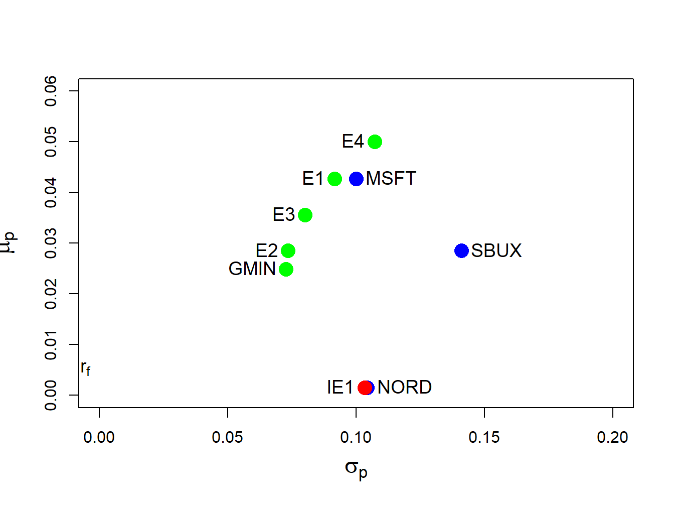
Figure 12.6: Minimum variance portfolios created as convex combinations of two minimum variance portfolios. Portfolios E3, E4 and IE1 are created from portfolios E1 and E2.
12.4.1 Algorithm for computing efficient frontier
The efficient frontier of portfolios, i.e., those frontier portfolios with expected return greater than the expected return on the global minimum variance portfolio, can be conveniently created using (12.22) with two specific efficient portfolios. The first efficient portfolio is the global minimum variance portfolio (12.2). The second efficient portfolio is the efficient portfolio whose target expected return is equal to the highest expected return among all of the assets under consideration. The choice of these two efficient portfolios makes it easy to produce a nice plot of the efficient frontier. The steps for constructing the efficient frontier are:
- Compute the global minimum variance portfolio \(\mathbf{m}\) by solving (12.2), and compute \(\mu_{p,m}=\mathbf{m}^{\prime}\mu\) and \(\sigma_{p,m}^{2}=\mathbf{m}^{\prime}\Sigma \mathbf{m}\).
- Compute the efficient portfolio \(\mathbf{x}\) with target expected return equal to the maximum expected return of the assets under consideration. That is, solve (12.10) with \(\mu_{0}=\max\{\mu_{1},\ldots,\mu_{N}\}\), and compute \(\mu_{p,x}=\mathbf{x}^{\prime}\mu\) and \(\sigma_{p,x}^{2}=\mathbf{x}^{\prime}\Sigma \mathbf{x}\).
- Compute \(\mathrm{cov}(R_{p,m},R_{p,x})=\sigma_{mx}=\mathbf{m}^{\prime}\Sigma \mathbf{x}\).
- Create an initial grid of \(\alpha\) values \(\{0,0.1,\ldots0.9,1\}\), and compute the frontier portfolios \(\mathbf{z}\) using \[ \mathbf{z}=\alpha\times\mathbf{x}+(1-\alpha)\times\mathbf{m}, \] and compute their expected returns and variances using (12.22), (12.23) and (12.24), respectively.
- Plot \(\mu_{p,z}\) against \(\sigma_{p,z}\) and adjust the grid of \(\alpha\) values appropriately to create a nice plot. Negative values of \(\alpha\) will give inefficient frontier portfolios. Values of \(\alpha\) greater than one will give efficient frontier portfolios with expected returns greater than \(\mu_{0}.\)
To compute the efficient frontier from the three risky assets in Table 12.1 in R use:
a = seq(from=0, to=1, by=0.1)
n.a = length(a)
z.mat = matrix(0, n.a, 3)
colnames(z.mat) = names(mu.vec)
mu.z = rep(0, n.a)
sig2.z = rep(0, n.a)
sig.mx = t(m.vec)%*%sigma.mat%*%x.vec
for (i in 1:n.a) {
   z.mat[i, ] = a[i]*x.vec + (1-a[i])*m.vec
   mu.z[i] = a[i]*mu.px + (1-a[i])*mu.gmin
   sig2.z[i] = a[i]^2 * sig2.px + (1-a[i])^2 * sig2.gmin +
      2*a[i]*(1-a[i])*sig.mx
}
The variables z.mat, mu.z and sig2.z contain
the weights, expected returns and variances, respectively, of the
efficient frontier portfolios for a grid of \(\alpha\) values between
0 and 1. The resulting efficient frontier is illustrated in Figure
12.7 created with:
plot(sqrt(sig2.z), mu.z, type="b", ylim=c(0, 0.06), xlim=c(0, 0.16),
     pch=16, col="green", cex = cex.val, ylab=expression(mu[p]),
     xlab=expression(sigma[p]),cex.lab=1.5)
points(sd.vec, mu.vec, pch=16, cex=2, lwd=2, col="blue")
points(sig.gmin, mu.gmin, pch=16, col="green", cex=2)
points(sig.px, mu.px, pch=16, col="green", cex=2)
text(sig.gmin, mu.gmin, labels="GLOBAL MIN", pos=2, cex = cex.val)
text(sd.vec, mu.vec, labels=asset.names, pos=4, cex = cex.val)
text(sig.px, mu.px, labels="E1", pos=2, cex = cex.val)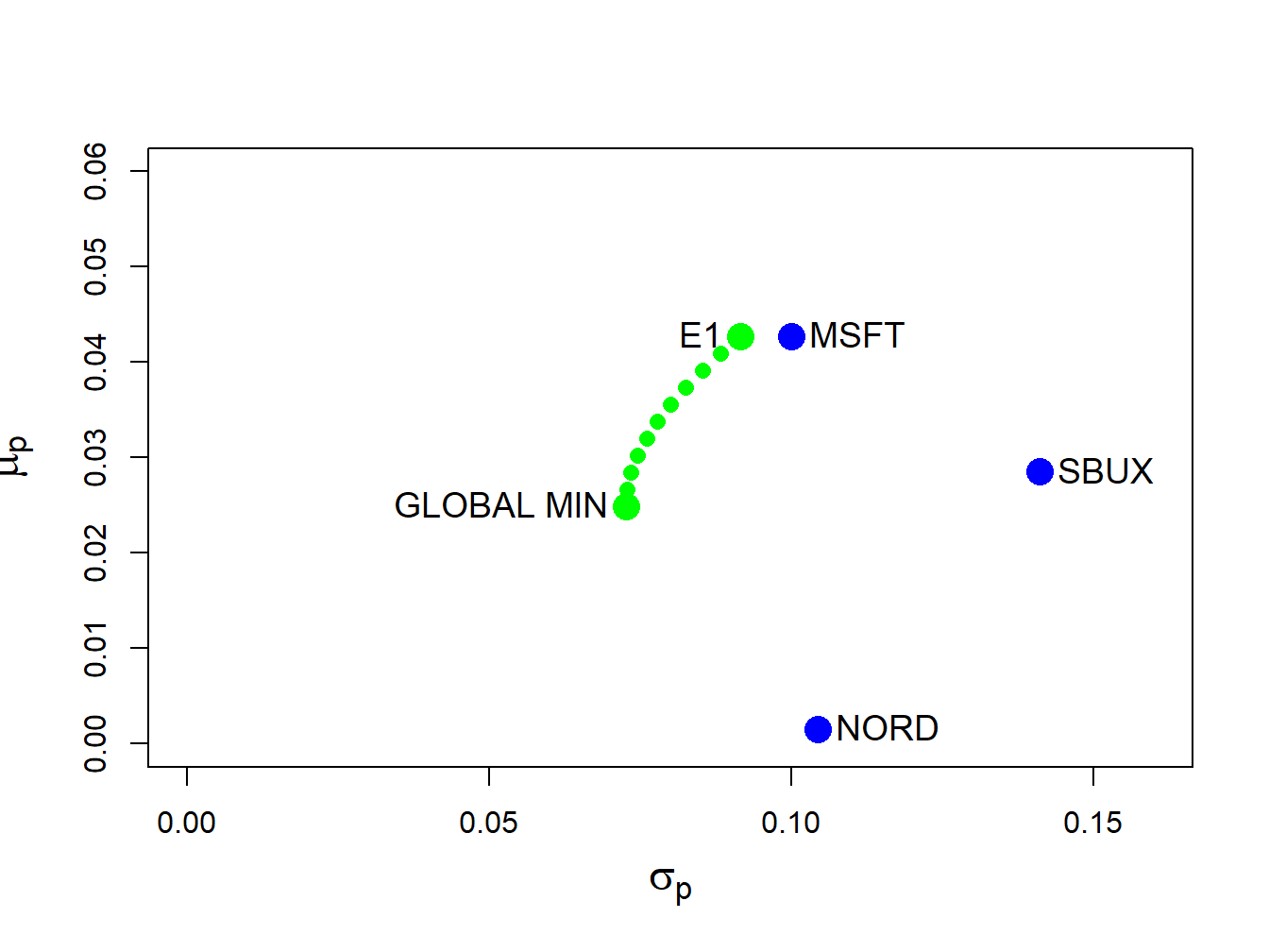
Figure 12.7: Efficient frontier computed from example data.
Each point on the efficient frontier is a portfolio of Microsoft,
Nordstrom and Starbucks. It is instructive to visualize the weights
in these portfolios as we move along the frontier from the global
minimum variance portfolio to the efficient portfolio with expected
return equal to the expected return on Microsoft. We can do this easily
using the PerformanceAnalytics function chart.StackedBar():
chart.StackedBar(z.mat, xaxis.labels=round(sqrt(sig2.z),digits=3),
                 legend.loc="upper",
                 colorset=rainbow8equal[1:3], ylab="Weights")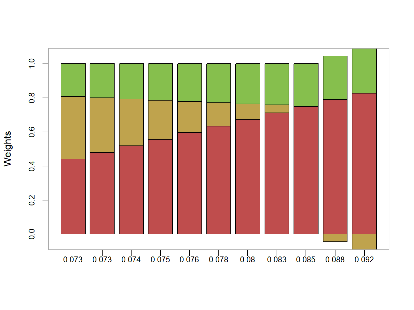
Figure 12.8: Portfolio weights in efficient frontier portfolios. x-axis is portfolio standard deviation
The resulting plot is shown in Figure 12.8. As we move along the frontier, the allocation to Microsoft increases and the allocation to Nordstrom decreases whereas the allocation to Starbucks stays about the same.
\(\blacksquare\)