2.1 Random Variables
We start with the basic definition of a random variable:
Definition 2.1 A random variable, \(X\), is a variable that can take on a given set of values, called the sample space and denoted \(S_{X}\), where the likelihood of the values in \(S_{X}\) is determined by \(X\)’s probability distribution function (pdf).
Consider the price of Microsoft stock next month, \(P_{t+1}\). Since \(P_{t+1}\) is not known with certainty today (\(t\)), we can consider it as a random variable. \(P_{t+1}\) must be positive, and realistically it can’t get too large. Therefore, the sample space is the set of positive real numbers bounded above by some large number: \(S_{P_{t+1}}=\{P_{t+1}:P_{t+1}\in[0,M],~M>0\}\). It is an open question as to what is the best characterization of the probability distribution of stock prices. The log-normal distribution is one possibility.9
\(\blacksquare\)
Consider a one-month investment in Microsoft stock. That is, we buy one share of Microsoft stock at the end of month \(t-1\) (e.g., end of February) and plan to sell it at the end of month \(t\) (e.g., end of March). The simple return over month \(t\) on this investment, \(R_{t}=(P_{t}-P_{t-1})/P_{t-1}\), is a random variable because we do not know what the price will be at the end of the month. In contrast to prices, returns can be positive or negative and are bounded from below by -100%. We can express the sample space as \(S_{R_{t}}=\{R_{t}:R_{t}\in[-1,M],~M>0\}\). The normal distribution is often a good approximation to the distribution of simple monthly returns, and is a better approximation to the distribution of continuously compounded monthly returns.
\(\blacksquare\)
As a final example, consider a variable \(X_{t+1}\) defined to be equal to one if the monthly price change on Microsoft stock, \(P_{t+1}-P_{t}\), is positive, and is equal to zero if the price change is zero or negative. Here, the sample space is the set \(S_{X_{t+1}}=\{0,1\}\). If it is equally likely that the monthly price change is positive or negative (including zero) then the probability that \(X_{t+1}=1\) or \(X_{t+1}=0\) is 0.5. This is an example of a Bernoulli random variable.
\(\blacksquare\)
The next sub-sections define discrete and continuous random variables.
2.1.1 Discrete random variables
Consider a random variable generically denoted \(X\) and its set of possible values or sample space denoted \(S_{X}\).
Definition 2.2 A discrete random variable \(X\) is one that can take on a finite number of \(n\) different values \(S_{X}=\{x_{1},x_{2},\ldots,x_{n}\}\) or, at most, a countably infinite number of different values \(S_{X}=\{x_{1},x_{2},\ldots.\}\).
Definition 2.3 The pdf of a discrete random variable, denoted \(p(x)\), is a function such that \(p(x)=\Pr(X=x)\). The pdf must satisfy (i) \(p(x)\geq0\) for all \(x\in S_{X}\); (ii) \(p(x)=0\) for all \(x\notin S_{X}\); and (iii) \(\sum_{x\in S_{X}}p(x)=1\).
| State of Economy | Sample Space | \(\Pr(X=x)\) |
|---|---|---|
| Depression | -0.30 | 0.05 |
| Recession | 0.0 | 0.20 |
| Normal | 0.10 | 0.50 |
| Mild Boom | 0.20 | 0.20 |
| Major Boom | 0.50 | 0.05 |
Let \(X\) denote the annual return on Microsoft stock over the next year. We might hypothesize that the annual return will be influenced by the general state of the economy. Consider five possible states of the economy: depression, recession, normal, mild boom and major boom. A stock analyst might forecast different values of the return for each possible state. Hence, \(X\) is a discrete random variable that can take on five different values. Table 2.1 describes such a probability distribution of the return and a graphical representation of the probability distribution is presented in Figure 2.1 created with
r.msft = c(-0.3, 0, 0.1, 0.2, 0.5)
prob.vals = c(0.05, 0.20, 0.50, 0.20, 0.05)
plot(r.msft, prob.vals, type="h", lwd=4, xlab="annual return",
     ylab="probability", xaxt="n")
points(r.msft, prob.vals, pch=16, cex=2, col="blue")
axis(1, at=r.msft)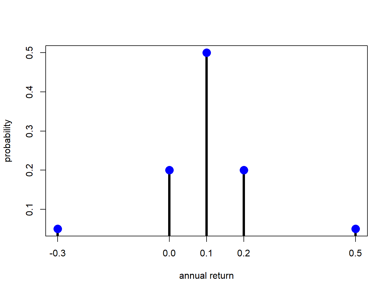
Figure 2.1: Discrete distribution for Microsoft stock.
The shape of the distribution is revealing. The center and most likely value is at \(0.1\) and the distribution is symmetric about this value (has the same shape to the left and to the right). Most of the probability is concentrated between \(0\) and \(0.2\) and there is very little probability associated with very large or small returns.
\(\blacksquare\)
2.1.1.1 The Bernoulli distribution
Let \(X=1\) if the price next month of Microsoft stock goes up and \(X=0\) if the price goes down (assuming it cannot stay the same). Then \(X\) is clearly a discrete random variable with sample space \(S_{X}=\{0,1\}\). If the probability of the stock price going up or down is the same then \(p(0)=p(1)=1/2\) and \(p(0)+p(1)=1\).
The probability distribution described above can be given an exact mathematical representation known as the Bernoulli distribution. Consider two mutually exclusive events generically called “success” and “failure”. For example, a success could be a stock price going up or a coin landing heads and a failure could be a stock price going down or a coin landing tails. The process creating the success or failure is called a Bernoulli trial. In general, let \(X=1\) if success occurs and let \(X=0\) if failure occurs. Let \(\Pr(X=1)=\pi\), where \(0<\pi<1\), denote the probability of success. Then \(\Pr(X=0)=1-\pi\) is the probability of failure. A mathematical model describing this distribution is: \[\begin{equation} p(x)=\Pr(X=x)=\pi^{x}(1-\pi)^{1-x},~x=0,1.\tag{2.1} \end{equation}\] When \(x=0\), \(p(0)=\pi^{0}(1-\pi)^{1-0}=1-\pi\) and when \(x=1,p(1)=\pi^{1}(1-\pi)^{1-1}=\pi\).
2.1.1.2 The binomial distribution
Consider a sequence of independent Bernoulli trials with success probability \(\pi\) generating a sequence of 0-1 variables indicating failures and successes. A binomial random variable \(X\) counts the number of successes in \(n\) Bernoulli trials, and is denoted \(X\sim B(n,\pi)\). The sample space is \(S_{X}=\{0,1,\ldots,n\}\) and: \[ \Pr(X=k)=\binom{n}{k}\pi^{k}(1-\pi)^{n-k}. \] The term \(\binom{n}{k}\) is the binomial coefficient, and counts the number of ways \(k\) objects can be chosen from \(n\) distinct objects. It is defined by: \[ \binom{n}{k}=\frac{n!}{(n-k)!k!}, \] where \(n!\) is the factorial of \(n\), or \(n(n-1)\cdots2\cdot1\).
2.1.2 Continuous random variables
A typical “bell-shaped” pdf is displayed in Figure 2.2 and the shaded area under the curve between -2 and 1 represents \(\Pr(-2\leq X \leq 1)\). For a continuous random variable, \(f(x)\neq\Pr(X=x)\) but rather gives the height of the probability curve at \(x\). In fact, \(\Pr(X=x)=0\) for all values of \(x\). That is, probabilities are not defined over single points. They are only defined over intervals. As a result, for a continuous random variable \(X\) we have: \[ \Pr(a\leq X\leq b)=\Pr(a<X\leq b)=\Pr(a<X<b)=\Pr(a\leq X<b). \]
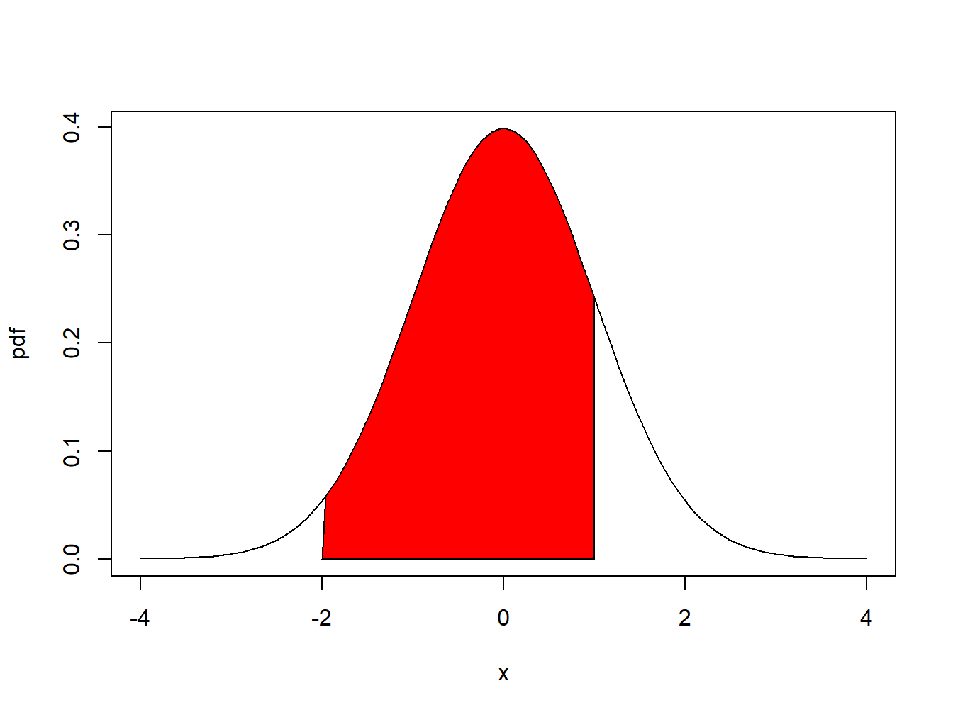
Figure 2.2: \(Pr(-2 \leq X \leq 1)\) is represented by the area under the probability curve.
2.1.2.1 The uniform distribution on an interval
Let \(X\) denote the annual return on Microsoft stock and let \(a\) and \(b\) be two real numbers such that \(a<b\). Suppose that the annual return on Microsoft stock can take on any value between \(a\) and \(b\). That is, the sample space is restricted to the interval \(S_{X}=\{x\in\mathcal{R}:a\leq x\leq b\}\). Further suppose that the probability that \(X\) will belong to any subinterval of \(S_{X}\) is proportional to the length of the interval. In this case, we say that \(X\) is uniformly distributed on the interval \([a,b]\). The pdf of \(X\) has a very simple mathematical form: \[ f(x)=\left\{ \begin{array}{c} \frac{1}{b-a}\\ 0 \end{array}\right.\begin{array}{c} \textrm{for }a\leq x\leq b,\\ \textrm{otherwise,} \end{array} \] and is presented graphically as a rectangle. It is easy to see that the area under the curve over the interval \([a,b]\) (area of rectangle) integrates to one: \[ \int_{a}^{b}\frac{1}{b-a}~dx=\frac{1}{b-a}\int_{a}^{b}~dx=\frac{1}{b-a}\left[x\right]_{a}^{b}=\frac{1}{b-a}[b-a]=1. \]
Let \(a=-1\) and \(b=1,\) so that \(b-a=2\). Consider computing the probability that \(X\) will be between -0.5 and 0.5. We solve: \[ \Pr(-0.5\leq X\leq0.5)=\int_{-0.5}^{0.5}\frac{1}{2}~dx=\frac{1}{2}\left[x\right]_{-0.5}^{0.5}=\frac{1}{2}\left[0.5-(-0.5)\right]=\frac{1}{2}. \] Next, consider computing the probability that the return will fall in the interval \([0,\delta]\) where \(\delta\) is some small number less than \(b=1\): \[ \Pr(0\leq X\leq\delta)=\frac{1}{2}\int_{0}^{\delta}dx=\frac{1}{2}[x]_{0}^{\delta}=\frac{1}{2}\delta. \] As \(\delta\rightarrow0\), \(\Pr(0\leq X\leq\delta)\rightarrow\Pr(X=0)\).
Using the above result we see that \[ \lim_{\delta\rightarrow0}\Pr(0\leq X\leq\delta)=\Pr(X=0)=\lim_{\delta\rightarrow0}\frac{1}{2}\delta=0. \] Hence, for continuous random variables probabilities are defined on intervals but not at distinct points.
\(\blacksquare\)
2.1.2.2 The standard normal distribution
The normal or Gaussian distribution is perhaps the most famous and most useful continuous distribution in all of statistics. The shape of the normal distribution is the familiar “bell curve”. As we shall see, it can be used to describe the probabilistic behavior of stock returns although other distributions may be more appropriate.
If a random variable \(X\) follows a standard normal distribution then we often write \(X\sim N(0,1)\) as short-hand notation. This distribution is centered at zero and has inflection points at \(\pm1\).10 The pdf of a standard normal random variable is given by: \[\begin{equation} f(x)=\frac{1}{\sqrt{2\pi}}\cdot e^{-\frac{1}{2}x^{2}},~-\infty\leq x\leq\infty.\tag{2.2} \end{equation}\] It can be shown via the change of variables formula in calculus that the area under the standard normal curve is one: \[ \int_{-\infty}^{\infty}\frac{1}{\sqrt{2\pi}}\cdot e^{-\frac{1}{2}x^{2}}dx=1. \] The standard normal distribution is illustrated in Figure 2.3. Notice that the distribution is symmetric about zero; i.e., the distribution has exactly the same form to the left and right of zero. Because the standard normal pdf formula is used so often it is given its own special symbol \(\phi(x)\).
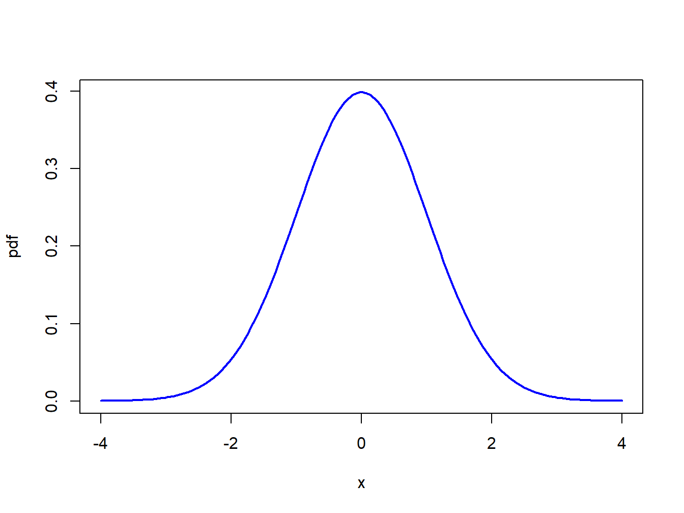
Figure 2.3: Standard normal density.
The normal distribution has the annoying feature that the area under the normal curve cannot be evaluated analytically. That is: \[ \Pr(a\leq X\leq b)=\int_{a}^{b}\frac{1}{\sqrt{2\pi}}\cdot e^{-\frac{1}{2}x^{2}}~dx, \] does not have a closed form solution. The above integral must be computed by numerical approximation. Areas under the normal curve, in one form or another, are given in tables in almost every introductory statistics book and standard statistical software can be used to find these areas. Some useful approximate results are: \[\begin{align*} \Pr(-1 & \leq X\leq1)\approx0.67,\\ \Pr(-2 & \leq X\leq2)\approx0.95,\\ \Pr(-3 & \leq X\leq3)\approx0.99. \end{align*}\]
2.1.3 The cumulative distribution function
The cdf has the following properties:
- If \(x_{1}<x_{2}\) then \(F_{X}(x_{1})\leq F_{X}(x_{2})\)
- \(F_{X}(-\infty)=0\) and \(F_{X}(\infty)=1\)
- \(\Pr(X>x)=1-F_{X}(x)\)
- \(\Pr(x_{1}<X\leq x_{2})=F_{X}(x_{2})-F_{X}(x_{1})\)
- \(F_{X}^{\prime}(x)=\frac{d}{dx}F_{X}(x)=f(x)\) if \(X\) is a continuous random variable and \(F_{X}(x)\) is continuous and differentiable.
The cdf for the discrete distribution of Microsoft from Table 2.1 is given by: \[ F_{X}(x)=\left\{ \begin{array}{c} 0,\\ 0.05,\\ 0.25,\\ 0.75\\ 0.95\\ 1 \end{array}\right.\begin{array}{c} x<-0.3\\ -0.3\leq x<0\\ 0\leq x<0.1\\ 0.1\leq x<0.2\\ 0.2\leq x<0.5\\ x>0.5 \end{array} \] and is illustrated in Figure 2.4.
\(\blacksquare\)
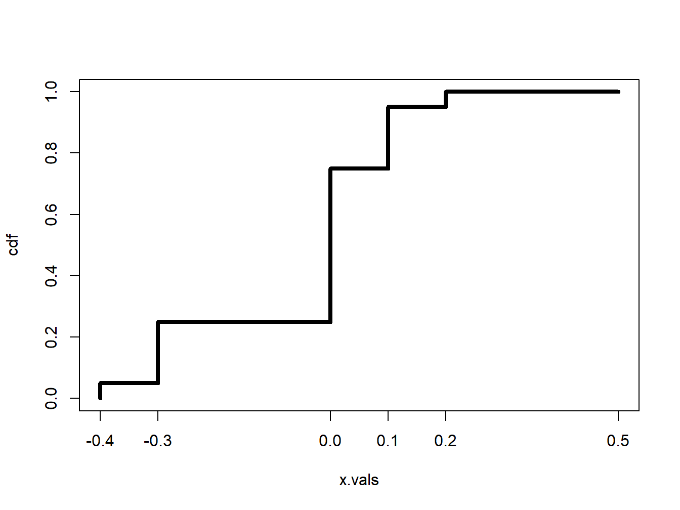
Figure 2.4: CDF of Discrete Distribution for Microsoft Stock Return.
The cdf for the uniform distribution over \([a,b]\) can be determined analytically: \[\begin{align*} F_{X}(x) & =\Pr(X<x)=\int_{-\infty}^{x}f(t)~dt\\ & =\frac{1}{b-a}\int_{a}^{x}~dt=\frac{1}{b-a}[t]_{a}^{x}=\frac{x-a}{b-a}. \end{align*}\] We can determine the pdf of \(X\) directly from the cdf via, \[ f(x)=F_{X}^{\prime}(x)=\frac{d}{dx}F_{X}(x)=\frac{1}{b-a}. \]
\(\blacksquare\)
The cdf of standard normal random variable \(X\) is used so often in statistics that it is given its own special symbol: \[\begin{equation} \Phi(x)=F_{X}(x)=\int_{-\infty}^{x}\frac{1}{\sqrt{2\pi}}e^{-\frac{1}{2}z^{2}}~dz.\tag{2.3} \end{equation}\] The cdf \(\Phi(x)\), however, does not have an analytic representation like the cdf of the uniform distribution and so the integral in (2.3) must be approximated using numerical techniques. A graphical representation of \(\Phi(x)\) is given in Figure 2.5. Because the standard normal pdf, \(\phi(x)\), is symmetric about zero and bell-shaped the standard normal CDF, \(\Phi(x)\), has an “S” shape where the middle of the “S” is at zero.
\(\blacksquare\)
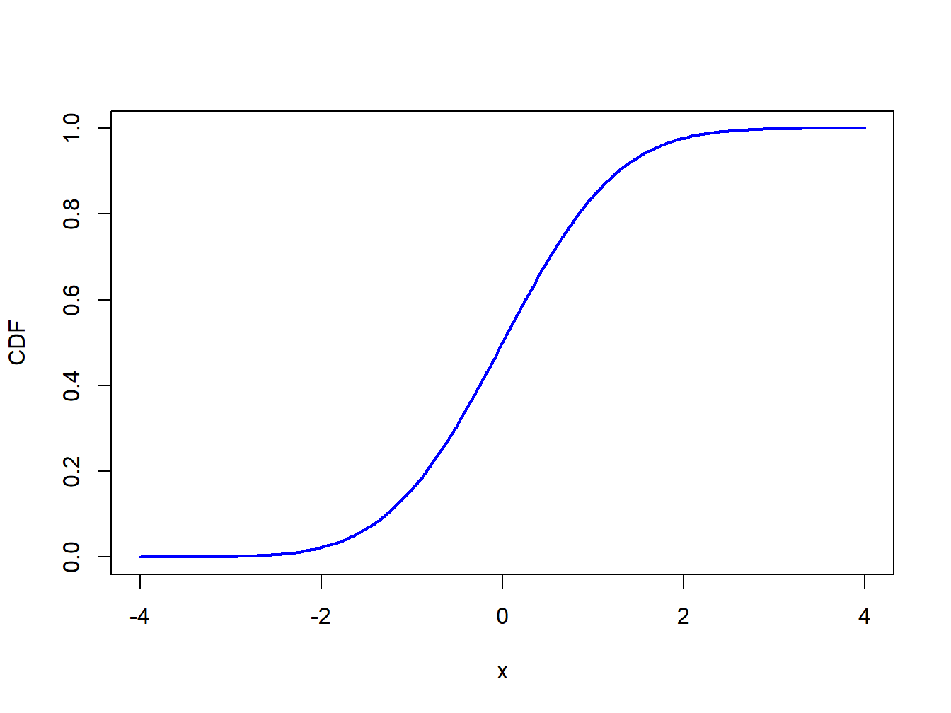
Figure 2.5: Standard normal cdf \(\Phi(x)\).
2.1.4 Quantiles of the distribution of a random variable
Definition 2.7 Consider a random variable \(X\) with continuous cdf \(F_{X}(x)\). For \(0\leq\alpha\leq1\), the \(100\cdot\alpha\%\) quantile of the distribution for \(X\) is the value \(q_{\alpha}\) that satisfies: \[ F_{X}(q_{\alpha})=\Pr(X\leq q_{\alpha})=\alpha. \] For example, the 5% quantile of \(X\), \(q_{0.05}\), satisfies, \[ F_{X}(q_{0.05})=\Pr(X\leq q_{0.05})=0.05. \]
The median of the distribution is the 50% quantile. That is, the median, \(q_{0.5}\), satisfies, \[ F_{X}(q_{0.5})=\Pr(X\leq q_{0.5})=0.5. \]
If \(F_{X}\) is invertible then \(q_{\alpha}\) may be determined analytically as: \[\begin{equation} q_{\alpha}=F_{X}^{-1}(\alpha)\tag{2.4} \end{equation}\] where \(F_{X}^{-1}\) denotes the inverse function of \(F_{X}\).11 Hence, the 5% quantile and the median may be determined from \[ q_{0.05}=F_{X}^{-1}(.05),q_{0.5}=F_{X}^{-1}(.5). \] The inverse cdf \(F_{X}^{-1}\) is sometimes called the quantile function.
Let \(X\sim U[a,b]\) where \(b>a\). Recall, the cdf of \(X\) is given by: \[ F_{X}(x)=\frac{x-a}{b-a},~a\leq x\leq b, \] which is continuous and strictly increasing. Given \(\alpha\in[0,1]\) such that \(F_{X}(x)=\alpha\), solving for \(x\) gives the inverse cdf: \[\begin{equation} x=F_{X}^{-1}(\alpha)=\alpha(b-a)+a.\tag{2.5} \end{equation}\] Using (2.5), the 5% quantile and median, for example, are given by: \[\begin{align*} q_{0.05} & =F_{X}^{-1}(.05)=.05(b-a)+a=.05b+.95a,\\ q_{0.5} & =F_{X}^{-1}(.5)=.5(b-a)+a=.5(a+b). \end{align*}\] If \(a=0\) and \(b=1\), then \(q_{0.05}=0.05\) and \(q_{0.5}=0.5\).
\(\blacksquare\)
Let \(X\sim N(0,1).\) The quantiles of the standard normal distribution are determined by solving \[\begin{equation} q_{\alpha}=\Phi^{-1}(\alpha),\tag{2.6} \end{equation}\] where \(\Phi^{-1}\) denotes the inverse of the cdf \(\Phi\). This inverse function must be approximated numerically and is available in most spreadsheets and statistical software. Using the numerical approximation to the inverse function, the 1%, 2.5%, 5%, 10% quantiles and median are given by: \[\begin{align*} q_{0.01} & =\Phi^{-1}(.01)=-2.33,~q_{0.025}=\Phi^{-1}(.025)=-1.96,\\ q_{0.05} & =\Phi^{-1}(.05)=-1.645,~q_{0.10}=\Phi^{-1}(.10)=-1.28,\\ q_{0.5} & =\Phi^{-1}(.5)=0. \end{align*}\] Often, the standard normal quantile is denoted \(z_{\alpha}\).
\(\blacksquare\)
2.1.5 R functions for discrete and continuous distributions
R has built-in functions for a number of discrete and continuous distributions
that are commonly used in probability modeling and statistical analysis.
These are summarized in Table 2.2.
For each distribution, there are four functions starting with d,
p, q, and r that compute density
(pdf) values, cumulative probabilities (cdf), quantiles
(inverse cdf) and random draws, respectively. Consider, for
example, the functions associated with the normal distribution. The
functions dnorm(), pnorm() and qnorm()
evaluate the standard normal density (2.2),
the cdf (2.3), and the inverse cdf or quantile
function (2.6), respectively, with
the default values mean = 0 and sd = 1. The function
rnorm() returns a specified number of simulated values from
the normal distribution.
| Distribution | Function (root) | Parameters | Defaults |
|---|---|---|---|
| beta | beta |
shape1, shape2 | _, _ |
| binomial | binom |
size, prob | _, _ |
| cauchy | cauchy |
location, scale | 0, 1 |
| chi-squared | chisq |
df, ncp | _, 1 |
| F | f |
df1, df2 | _, _ |
| gamma | gamma |
shape, rate, scale | _, 1, 1/rate |
| geometric | geom |
prob | _ |
| hyper-geometric | hyper |
m, n, k | _, _, _ |
| log-normal | lnorm |
meanlog, sdlog | 0, 1 |
| logistic | logis |
location, scale | 0, 1 |
| negative binomial | nbinom |
size, prob, mu | _,_,_ |
| normal | norm |
mean, sd | 0, 1 |
| Poisson | pois |
Lambda | 1 |
| Student’s t | t |
df, ncp | _, 1 |
| uniform | unif |
min, max | 0, 1 |
| Weibull | weibull |
shape, scale | _, 1 |
| Wilcoxon | wilcoxon |
m, n | _, _ |
Commonly used distributions used in finance application are the binomial, chi-squared, log normal, normal, and Student’s t.
2.1.5.1 Finding areas under the standard normal curve
Let \(X\) denote a standard normal random variable. Given that the total area under the normal curve is one and the distribution is symmetric about zero, the following results hold:
- \(\Pr(X\leq z)=1-\Pr(X\geq z)\) and \(\Pr(X\geq z)=1-\Pr(X\leq z)\)
- \(\Pr(X\geq z)=\Pr(X\leq-z)\)
- \(\Pr(X\geq0)=\Pr(X\leq0)=0.5\)
The following examples show how to do probability calculations with standard normal random variables.
First, consider finding \(\Pr(X\geq2)\). By the symmetry of the normal distribution, \(\Pr(X\geq2)=\Pr(X\leq-2)=\Phi(-2)\). In R use:
## [1] 0.02275013Next, consider finding \(\Pr(-1\leq X\leq2)\). Using the cdf, we compute \(\Pr(-1\leq X\leq2)=\Pr(X\leq2)-\Pr(X\leq-1)=\Phi(2)-\Phi(-1)\). In R use:
## [1] 0.8185946Finally, using R the exact values for \(\Pr(-1\leq X\leq1)\), \(\Pr(-2\leq X\leq2)\) and \(\Pr(-3\leq X\leq3)\) are:
## [1] 0.6826895## [1] 0.9544997## [1] 0.9973002\(\blacksquare\)
2.1.5.2 Plotting distributions
When working with a probability distribution, it is a good idea to make plots of the pdf or cdf to reveal important characteristics. The following examples illustrate plotting distributions using R.
The graphs of the standard normal pdf and cdf in Figures 2.3 and 2.5 were created using the following R code:
# plot pdf
x.vals = seq(-4, 4, length=150)
plot(x.vals, dnorm(x.vals), type="l", lwd=2, col="blue",
     xlab="x", ylab="pdf")
# plot cdf
plot(x.vals, pnorm(x.vals), type="l", lwd=2, col="blue",
     xlab="x", ylab="CDF")
\(\blacksquare\)
Figure 2.2 showing \(\Pr(-2\leq X\leq1)\) as a red shaded area is created with the following code:
lb = -2
ub = 1
x.vals = seq(-4, 4, length=150)
d.vals = dnorm(x.vals)
# plot normal density
plot(x.vals, d.vals, type="l", xlab="x", ylab="pdf")
i = x.vals >= lb & x.vals <= ub
# add shaded region between -2 and 1
polygon(c(lb, x.vals[i], ub), c(0, d.vals[i], 0), col="red")
\(\blacksquare\)
2.1.6 Shape characteristics of probability distributions
Very often we would like to know certain shape characteristics of a probability distribution. We might want to know where the distribution is centered, and how spread out the distribution is about the central value. We might want to know if the distribution is symmetric about the center or if the distribution has a long left or right tail. For stock returns we might want to know about the likelihood of observing extreme values for returns representing market crashes. This means that we would like to know about the amount of probability in the extreme tails of the distribution. In this section we discuss four important shape characteristics of a probability distribution:
- expected value (mean): measures the center of mass of a distribution
- variance and standard deviation (volatility): measures the spread about the mean
- skewness: measures symmetry about the mean
- kurtosis: measures “tail thickness”
2.1.6.1 Expected Value
The expected value of a random variable \(X,\) denoted \(E[X]\) or \(\mu_{X}\), measures the center of mass of the pdf.
Equation (2.7) shows that \(E[X]\) is a probability weighted average of the possible values of \(X\).
Using the discrete distribution for the return on Microsoft stock in Table 2.1, the expected return is computed as: \[\begin{align*} E[X] =&(-0.3)\cdot(0.05)+(0.0)\cdot(0.20)+(0.1)\cdot(0.5)\\ &+(0.2)\cdot(0.2)+(0.5)\cdot(0.05)\\ =&0.10. \end{align*}\]
\(\blacksquare\)
Let \(X\) be a Bernoulli random variable with success probability \(\pi\). Then, \[ E[X]=0\cdot(1-\pi)+1\cdot\pi=\pi. \] That is, the expected value of a Bernoulli random variable is its probability of success. Now, let \(Y\sim B(n,\pi)\). It can be shown that: \[\begin{equation} E[Y]=\sum_{k=0}^{n}k\binom{n}{k}\pi^{k}(1-\pi)^{n-k}=n\pi.\tag{2.8} \end{equation}\]
\(\blacksquare\)
Definition 2.9 For a continuous random variable \(X\) with pdf \(f(x)\), the expected value is defined as: \[\begin{equation} \mu_{X}=E[X]=\int_{-\infty}^{\infty}x\cdot f(x)~dx.\tag{2.9} \end{equation}\]
Suppose \(X\) has a uniform distribution over the interval \([a,b]\). Then, \[\begin{align*} E[X] & =\frac{1}{b-a}\int_{a}^{b}x~dx=\frac{1}{b-a}\left[\frac{1}{2}x^{2}\right]_{a}^{b}\\ & =\frac{1}{2(b-a)}\left[b^{2}-a^{2}\right]\\ & =\frac{(b-a)(b+a)}{2(b-a)}=\frac{b+a}{2}. \end{align*}\] If \(b=-1\) and \(a=1\), then \(E[X]=0\).
\(\blacksquare\)
Let \(X\sim N(0,1)\). Then it can be shown that: \[ E[X]=\int_{-\infty}^{\infty}x\cdot\frac{1}{\sqrt{2\pi}}e^{-\frac{1}{2}x^{2}}~dx=0. \] Hence, the standard normal distribution is centered at zero.
\(\blacksquare\)
2.1.6.2 Expectation of a function of a random variable
The other shape characteristics of the distribution of a random variable \(X\) are based on expectations of certain functions of \(X\).
2.1.6.3 Variance and standard deviation
The variance of a random variable \(X\), denoted \(\mathrm{var}(X)\) or \(\sigma_{X}^{2}\), measures the spread of the distribution about the mean using the function \(g(X)=(X-\mu_{X})^{2}\). If most values of \(X\) are close to \(\mu_{X}\) then on average \((X-\mu_{X})^{2}\) will be small. In contrast, if many values of \(X\) are far below and/or far above \(\mu_{X}\) then on average \((X-\mu_{X})^{2}\) will be large. Squaring the deviations about \(\mu_{X}\) guarantees a positive value.
Definition 2.11 For a discrete or continuous random variable \(X\), the variance and standard deviation of \(X\) are defined as: \[\begin{align} \sigma_{X}^{2}&=\mathrm{var}(X)=E[(X-\mu_{X})^{2}],\tag{2.12} \\ \sigma_{X} &= \mathrm{sd}(X)= \sqrt{\sigma_{X}^{2}} = \sigma_{X}. \tag{2.13} \end{align}\]
Because \(\sigma_{X}^{2}\) represents an average squared deviation, it is not in the same units as \(X\). The standard deviation of \(X\) is the square root of the variance and is in the same units as \(X\). For “bell-shaped” distributions, \(\sigma_{X}\) measures the typical size of a deviation from the mean value.
The computation of (2.12) can often be simplified by using the result: \[\begin{equation} \mathrm{var}(X)=E[(X-\mu_{X})^{2}]=E[X^{2}]-\mu_{X}^{2}\tag{2.14} \end{equation}\] We will learn how to derive this result later in the chapter.
Using the discrete distribution for the return on Microsoft stock in Table 2.1 and the result that \(\mu_{X}=0.1\), we have: \[\begin{align*} \mathrm{var}(X) & =(-0.3-0.1)^{2}\cdot(0.05)+(0.0-0.1)^{2}\cdot(0.20)+(0.1-0.1)^{2}\cdot(0.5)\\ & +(0.2-0.1)^{2}\cdot(0.2)+(0.5-0.1)^{2}\cdot(0.05)\\ & =0.020. \end{align*}\] Alternatively, we can compute \(\mathrm{var}(X)\) using (2.14): \[\begin{align*} E[X^{2}]-\mu_{X}^{2} & =(-0.3)^{2}\cdot(0.05)+(0.0)^{2}\cdot(0.20)+(0.1)^{2}\cdot(0.5)\\ & +(0.2)^{2}\cdot(0.2)+(0.5)^{2}\cdot(0.05)-(0.1)^{2}\\ & =0.020. \end{align*}\] The standard deviation is \(\sqrt{0.020}=0.141\). Given that the distribution is fairly bell-shaped we can say that typical values deviate from the mean value of \(10\%\) by about \(\pm 14.1\%\).
\(\blacksquare\)
Let \(X\) be a Bernoulli random variable with success probability \(\pi\). Given that \(\mu_{X}=\pi\) it follows that: \[\begin{align*} \mathrm{var}(X) & =(0-\pi)^{2}\cdot(1-\pi)+(1-\pi)^{2}\cdot\pi\\ & =\pi^{2}(1-\pi)+(1-\pi)^{2}\pi\\ & =\pi(1-\pi)\left[\pi+(1-\pi)\right]\\ & =\pi(1-\pi),\\ \mathrm{sd}(X) & =\sqrt{\pi(1-\pi)}. \end{align*}\] Now, let \(Y\sim B(n,\pi)\): It can be shown that: \[ \mathrm{var}(Y)=n\pi(1-\pi) \] and so \(\mathrm{sd}(Y)=\sqrt{n\pi(1-\pi)}\).
\(\blacksquare\)
Let \(X\sim U[a,b]\). Using (2.14) and \(\mu_{X}=\frac{a+b}{2}\), after some algebra, it can be shown that: \[ \mathrm{var}(X)=E[X^{2}]-\mu_{X}^{2}=\frac{1}{b-a}\int_{a}^{b}x^{2}~dx-\left(\frac{a+b}{2}\right)^{2}=\frac{1}{12}(b-a)^{2}, \] and \(\mathrm{sd}(X)=(b-a)/\sqrt{12}\).
\(\blacksquare\)
Let \(X\sim N(0,1)\). Here, \(\mu_{X}=0\) and it can be shown that: \[ \sigma_{X}^{2}=\int_{-\infty}^{\infty}x^{2}\cdot\frac{1}{\sqrt{2\pi}}e^{-\frac{1}{2}x^{2}}~dx=1. \] It follows that sd\((X)=1\).
\(\blacksquare\)
2.1.6.4 The general normal distribution
Recall, if \(X\) has a standard normal distribution then \(E[X]=0\), \(\mathrm{var}(X)=1\). A general normal random variable \(X\) has \(E[X]=\mu_{X}\) and \(\mathrm{var}(X)=\sigma_{X}^{2}\) and is denoted \(X\sim N(\mu_{X},\sigma_{X}^{2})\). Its pdf is given by: \[\begin{equation} f(x)=\frac{1}{\sqrt{2\pi\sigma_{X}^{2}}}\exp\left\{ -\frac{1}{2\sigma_{X}^{2}}\left(x-\mu_{X}\right)^{2}\right\} ,~-\infty\leq x\leq\infty.\tag{2.15} \end{equation}\] Showing that \(E[X]=\mu_{X}\) and \(\mathrm{var}(X)=\sigma_{X}^{2}\) is a bit of work and is good calculus practice. As with the standard normal distribution, areas under the general normal curve cannot be computed analytically. Using numerical approximations, it can be shown that: \[\begin{align*} \Pr(\mu_{X}-\sigma_{X} & <X<\mu_{X}+\sigma_{X})\approx0.67,\\ \Pr(\mu_{X}-2\sigma_{X} & <X<\mu_{X}+2\sigma_{X})\approx0.95,\\ \Pr(\mu_{X}-3\sigma_{X} & <X<\mu_{X}+3\sigma_{X})\approx0.99. \end{align*}\] Hence, for a general normal random variable about 95% of the time we expect to see values within \(\pm\) 2 standard deviations from its mean. Observations more than three standard deviations from the mean are very unlikely.
Let \(R\) denote the monthly return on an investment in Microsoft stock, and assume that it is normally distributed with mean \(\mu_{R}=0.01\) and standard deviation \(\sigma_{R}=0.10\). That is, \(R\sim N(0.01,(0.10)^{2})\). Notice that \(\sigma_{R}^{2}=0.01\) and is not in units of return per month. Figure 2.6 illustrates the distribution and is created using:
mu.r = 0.01
sd.r = 0.1
x.vals = seq(-4, 4, length=150)*sd.r + mu.r
plot(x.vals, dnorm(x.vals, mean=mu.r, sd=sd.r), type="l", lwd=2,
     col="blue", xlab="x", ylab="pdf")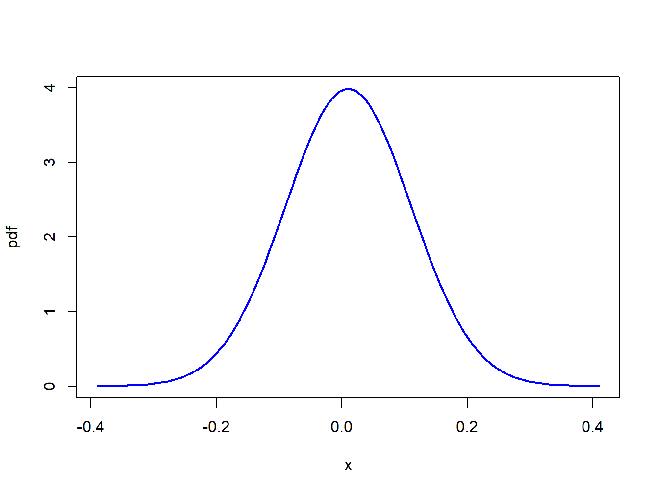
Figure 2.6: Normal distribution for the monthly returns on Microsoft: \(R\sim N(0.01,(0.10)^{2})\).
Notice that essentially all of the probability lies between \(-0.3\)
and \(0.3\). Using the R function pnorm(), we can easily compute
the probabilities \(\Pr(R<-0.5)\), \(\Pr(R<0)\), \(\Pr(R>0.5)\) and \(\Pr(R>1)\):
## [1] 1.698267e-07## [1] 0.4601722## [1] 4.791833e-07## [1] 0Using the R function , we can find the quantiles \(q_{0.01}\), \(q_{0.05}\), \(q_{0.95}\) and \(q_{0.99}\):
## [1] -0.2226348 -0.1544854 0.1744854 0.2426348Hence, over the next month, there are 1% and 5% chances of losing more than 22.2% and 15.5%, respectively. In addition, there are 5% and 1% chances of gaining more than 17.5% and 24.3%, respectively.
\(\blacksquare\)
Consider the following investment problem. We can invest in two non-dividend paying stocks, Amazon and Boeing, over the next month. Let \(R_{A}\) denote the monthly return on Amazon and \(R_{B}\) denote the monthly return on Boeing. Assume that \(R_{A}\sim N(0.02,(0.10)^{2})\) and \(R_{B}\sim N(0.01,(0.05)^{2})\). Figure 2.7 shows the pdfs for the two returns. Notice that \(\mu_{A}=0.02>\mu_{B}=0.01\) but also that \(\sigma_{A}=0.10>\sigma_{B}=0.05\). The return we expect on Amazon is bigger than the return we expect on Boeing but the variability of Amazon’s return is also greater than the variability of Boeing’s return. The high return variability (volatility) of Amazon reflects the higher risk associated with investing in Amazon compared to investing in Boeing. If we invest in Boeing we get a lower expected return, but we also get less return variability or risk. For example, the probability of losing more than \(10\%\) in one month for Amazon is
## [1] 0.1150697and the probability of losing more than \(10\%\) in one month for Boeing is
## [1] 0.01390345Of course, there is also a higher probability for upside return for Amazon than for Boeing. This example illustrates the fundamental “no free lunch” principle of economics and finance: you can’t get something for nothing. In general, to get a higher expected return you must be prepared to take on higher risk.
\(\blacksquare\)
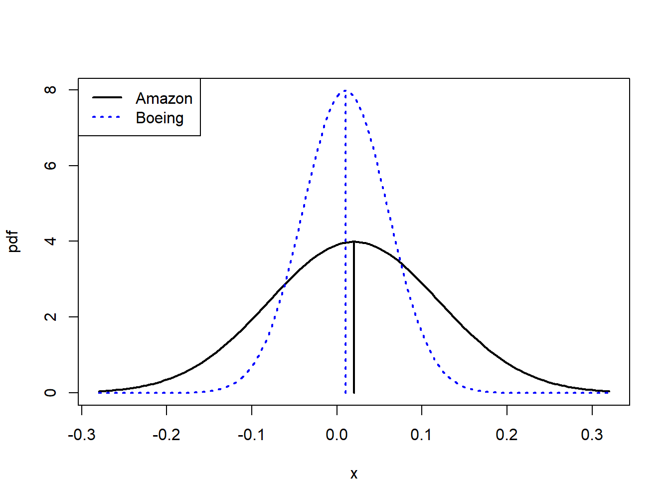
Figure 2.7: Risk-return tradeoff between one-month investments in Amazon and Boeing stock.
Let \(R_{t}\) denote the simple annual return on an asset, and suppose that \(R_{t}\sim N(0.05,(0.50)^{2})\). Because asset prices must be non-negative, \(R_{t}\) must always be larger than \(-1\). However, the normal distribution is defined for \(-\infty\leq R_{t}\leq\infty\) and based on the assumed normal distribution \(\Pr(R_{t}<-1)=0.018\). That is, there is a 1.8% chance that \(R_{t}\) is smaller than \(-1\). This implies that there is a 1.8% chance that the asset price at the end of the year will be negative! This is one reason why the normal distribution may not be appropriate for simple returns.
\(\blacksquare\)
Let \(r_{t}=\ln(1+R_{t})\) denote the continuously compounded annual return on an asset, and suppose that \(r_{t}\sim N(0.05,(0.50)^{2})\). Unlike the simple return, the continuously compounded return can take on values less than \(-1\). In fact, \(r_{t}\) is defined for \(-\infty\leq r_{t}\leq\infty\). For example, suppose \(r_{t}=-2\). This implies a simple return of \(R_{t}=e^{-2}-1=-0.865\). Then \(\Pr(r_{t}\leq-2)=\Pr(R_{t}\leq-0.865)=0.00002\). Although the normal distribution allows for values of \(r_{t}\) smaller than \(-1\), the implied simple return \(R_{t}\) will always be greater than \(-1\).
\(\blacksquare\)
2.1.6.5 The Log-Normal Distribution
Let \(X\) \(\sim N(\mu_{X},\sigma_{X}^{2})\), which is defined for \(-\infty<X<\infty\). The log-normally distributed random variable \(Y\) is determined from the normally distributed random variable \(X\) using the transformation \(Y=e^{X}\). In this case, we say that \(Y\) is log-normally distributed and write: \[\begin{equation} Y\sim\ln N(\mu_{X},\sigma_{X}^{2}),~0<Y<\infty.\tag{2.16} \end{equation}\] The pdf of the log-normal distribution for \(Y\) can be derived from the normal distribution for \(X\) using the change-of-variables formula from calculus and is given by: \[\begin{equation} f(y)=\frac{1}{y\sigma_{X}\sqrt{2\pi}}e^{-\frac{(\ln y-\mu_{X})^{2}}{2\sigma_{X}^{2}}}.\tag{2.17} \end{equation}\] Due to the exponential transformation, \(Y\) is only defined for non-negative values. It can be shown that: \[\begin{align} \mu_{Y} & =E[Y]=e^{\mu_{X}+\sigma_{X}^{2}/2},\tag{2.18}\\ \sigma_{Y}^{2} & =\mathrm{var}(Y)=e^{2\mu_{X}+\sigma_{X}^{2}}(e^{\sigma_{X}^{2}}-1).\nonumber \end{align}\]
Let \(r_{t}=\ln(P_{t}/P_{t-1})\) denote the continuously compounded monthly return on an asset and assume that \(r_{t}\sim N(0.05,(0.50)^{2})\). That is, \(\mu_{r}=0.05\) and \(\sigma_{r}=0.50\). Let \(R_{t}=(P_{t}-P_{t-1})/P_{t}\) denote the simple monthly return. The relationship between \(r_{t}\) and \(R_{t}\) is given by \(r_{t}=\ln(1+R_{t})\) and \(1+R_{t}=e^{r_{t}}\). Since \(r_{t}\) is normally distributed, \(1+R_{t}\) is log-normally distributed. Notice that the distribution of \(1+R_{t}\) is only defined for positive values of \(1+R_{t}\). This is appropriate since the smallest value that \(R_{t}\) can take on is \(-1\). Using (2.18), the mean and variance for \(1+R_{t}\) are given by: \[\begin{align*} \mu_{1+R} & =e^{0.05+(0.5)^{2}/2}=1.191\\ \sigma_{1+R}^{2} & =e^{2(0.05)+(0.5)^{2}}(e^{(0.5)^{2}}-1)=0.563 \end{align*}\] The pdfs for \(r_{t}\) and \(R_{t}\) are shown in Figure 2.8.
\(\blacksquare\)
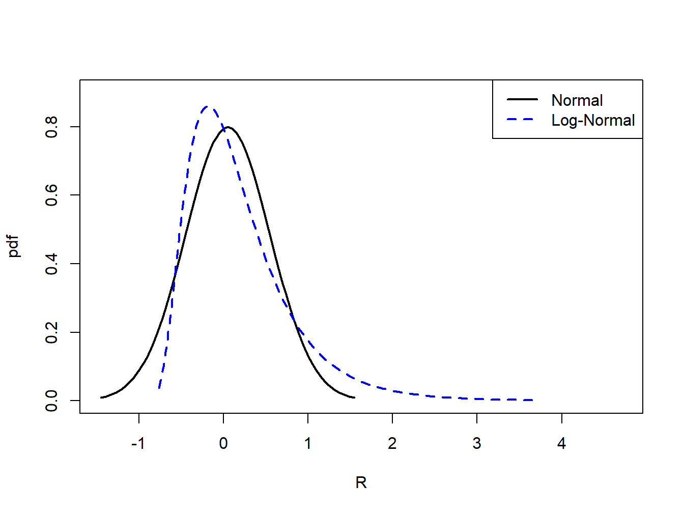
Figure 2.8: Normal distribution for \(r_{t}\) and log-normal distribution for \(R_{t}=e^{r_{t}}-1\).
2.1.6.6 Skewness
Definition 2.12 The skewness of a random variable \(X\), denoted \(\mathrm{skew}(X)\), measures the symmetry of a distribution about its mean value using the function \(g(X)=(X-\mu_{X})^{3}/\sigma_{X}^{3}\), where \(\sigma_{X}^{3}\) is just \(\mathrm{sd}(X)\) raised to the third power: \[\begin{equation} \mathrm{skew}(X)=\frac{E[(X-\mu_{X})^{3}]}{\sigma_{X}^{3}}\tag{2.19} \end{equation}\]
When \(X\) is far below its mean, \((X-\mu_{X})^{3}\) is a big negative number. When \(X\) is far above its mean, \((X-\mu_{X})^{3}\) is a big positive number. Hence, if there are more big values of \(X\) below \(\mu_{X}\) then \(\mathrm{skew}(X)<0\). Conversely, if there are more big values of \(X\) above \(\mu_{X}\) then \(\mathrm{skew}(X)>0\). If \(X\) has a symmetric distribution, then \(\mathrm{skew}(X)=0\) since positive and negative values in (2.19) cancel out. If \(\mathrm{skew}(X)>0\), then the distribution of \(X\) has a long right tail and if \(\mathrm{skew}(X)<0\) the distribution of \(X\) has a long left tail. These cases are illustrated in Figure 2.9.
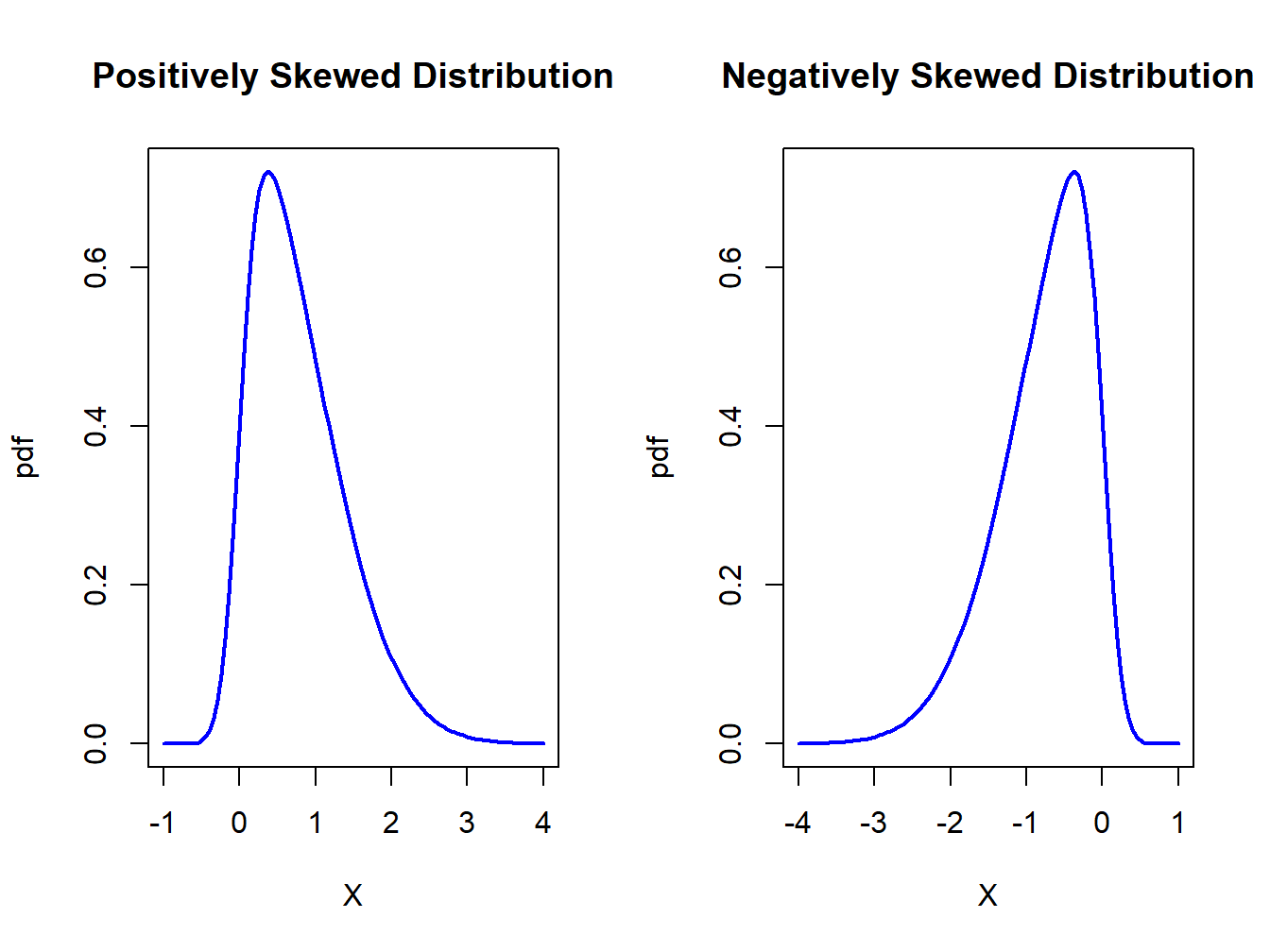
Figure 2.9: Skewed distributions.
Using the discrete distribution for the return on Microsoft stock in Table 2.1, the results that \(\mu_{X}=0.1\) and \(\sigma_{X}=0.141\), we have: \[\begin{align*} \mathrm{skew}(X) & =[(-0.3-0.1)^{3}\cdot(0.05)+(0.0-0.1)^{3}\cdot(0.20)+(0.1-0.1)^{3}\cdot(0.5)\\ & +(0.2-0.1)^{3}\cdot(0.2)+(0.5-0.1)^{3}\cdot(0.05)]/(0.141)^{3}\\ & =0.0. \end{align*}\]
\(\blacksquare\)
Suppose \(X\) has a general normal distribution with mean \(\mu_{X}\) and variance \(\sigma_{X}^{2}\). Then it can be shown that: \[ \mathrm{skew}(X)=\int_{-\infty}^{\infty}\frac{(x-\mu_{X})^{3}}{\sigma_{X}^{3}}\cdot\frac{1}{\sqrt{2\pi\sigma^{2}}}e^{-\frac{1}{2\sigma_{X}^{2}}\left(x-\mu_{X}\right)^{2}}~dx=0. \] This result is expected since the normal distribution is symmetric about it’s mean value \(\mu_{X}\).
\(\blacksquare\)
Let \(Y=e^{X},\) where \(X\sim N(\mu_{X},\sigma_{X}^{2})\), be a log-normally distributed random variable with parameters \(\mu_{X}\) and \(\sigma_{X}^{2}\). Then it can be shown that: \[ \mathrm{skew}(Y)=\left(e^{\sigma_{X}^{2}}+2\right)\sqrt{e^{\sigma_{X}^{2}}-1}>0. \] Notice that \(\mathrm{skew}(Y)\) is always positive, indicating that the distribution of \(Y\) has a long right tail, and that it is an increasing function of \(\sigma_{X}^{2}\). This positive skewness is illustrated in Figure 2.8.
\(\blacksquare\)
2.1.6.7 Kurtosis
Definition 2.13 The kurtosis of a random variable \(X\), denoted \(\mathrm{kurt}(X)\), measures the thickness in the tails of a distribution and is based on \(g(X)=(X-\mu_{X})^{4}/\sigma_{X}^{4}\): \[\begin{equation} \mathrm{kurt}(X)=\frac{E[(X-\mu_{X})^{4}]}{\sigma_{X}^{4}},\tag{2.20} \end{equation}\] where \(\sigma_{X}^{4}\) is just \(\mathrm{sd}(X)\) raised to the fourth power.
Since kurtosis is based on deviations from the mean raised to the fourth power, large deviations get lots of weight. Hence, distributions with large kurtosis values are ones where there is the possibility of extreme values. In contrast, if the kurtosis is small then most of the observations are tightly clustered around the mean and there is very little probability of observing extreme values.
Using the discrete distribution for the return on Microsoft stock in Table 2.1, the results that \(\mu_{X}=0.1\) and \(\sigma_{X}=0.141\), we have: \[\begin{align*} \mathrm{kurt}(X) & =[(-0.3-0.1)^{4}\cdot(0.05)+(0.0-0.1)^{4}\cdot(0.20)+(0.1-0.1)^{4}\cdot(0.5)\\ & +(0.2-0.1)^{4}\cdot(0.2)+(0.5-0.1)^{4}\cdot(0.05)]/(0.141)^{4}\\ & =6.5. \end{align*}\]
\(\blacksquare\)
Suppose \(X\) has a general normal distribution with mean \(\mu_{X}\) and variance \(\sigma_{X}^{2}\). Then it can be shown that: \[ \mathrm{kurt}(X)=\int_{-\infty}^{\infty}\frac{(x-\mu_{X})^{4}}{\sigma_{X}^{4}}\cdot\frac{1}{\sqrt{2\pi\sigma_{X}^{2}}}e^{-\frac{1}{2}(\frac{x-\mu_{X}}{\sigma_{X}})^{2}}~dx=3. \] Hence, a kurtosis of 3 is a benchmark value for tail thickness of bell-shaped distributions. If a distribution has a kurtosis greater than 3, then the distribution has thicker tails than the normal distribution. If a distribution has kurtosis less than 3, then the distribution has thinner tails than the normal.
\(\blacksquare\)
Sometimes the kurtosis of a random variable is described relative to the kurtosis of a normal random variable. This relative value of kurtosis is referred to as excess kurtosis and is defined as: \[\begin{equation} \mathrm{ekurt}(X)=\mathrm{kurt}(X)-3\tag{2.21} \end{equation}\] If the excess kurtosis of a random variable is equal to zero then the random variable has the same kurtosis as a normal random variable. If excess kurtosis is greater than zero, then kurtosis is larger than that for a normal; if excess kurtosis is less than zero, then kurtosis is less than that for a normal.
2.1.6.8 The Student’s t Distribution
The kurtosis of a random variable gives information on the tail thickness of its distribution. The normal distribution, with kurtosis equal to three, gives a benchmark for the tail thickness of symmetric distributions. A distribution similar to the standard normal distribution but with fatter tails, and hence larger kurtosis, is the Student’s t distribution. If \(X\) has a Student’s t distribution with degrees of freedom parameter \(v\), denoted \(X\sim t_{v},\) then its pdf has the form: \[\begin{equation} f(x)=\frac{\Gamma\left(\frac{v+1}{2}\right)}{\sqrt{v\pi}\Gamma\left(\frac{v}{2}\right)}\left(1+\frac{x^{2}}{v}\right)^{-\left(\frac{v+1}{2}\right)},~-\infty<x<\infty,~v>0.\tag{2.22} \end{equation}\] where \(\Gamma(z)=\int_{0}^{\infty}t^{z-1}e^{-t}dt\) denotes the gamma function. It can be shown that: \[\begin{align*} E[X] & =0,~v>1\\ \mathrm{var}(X) & =\frac{v}{v-2},~v>2,\\ \mathrm{skew}(X) & =0,~v>3,\\ \mathrm{kurt}(X) & =\frac{6}{v-4}+3,~v>4. \end{align*}\] The parameter \(v\) controls the scale and tail thickness of the distribution. If \(v\) is close to four, then the kurtosis is large and the tails are thick. If \(v<4\), then \(\mathrm{kurt}(X)=\infty\). As \(v\rightarrow\infty\) the Student’s t pdf approaches that of a standard normal random variable and \(\mathrm{kurt}(X)=3\). Figure 2.10 shows plots of the Student’s t density for various values of \(v\).
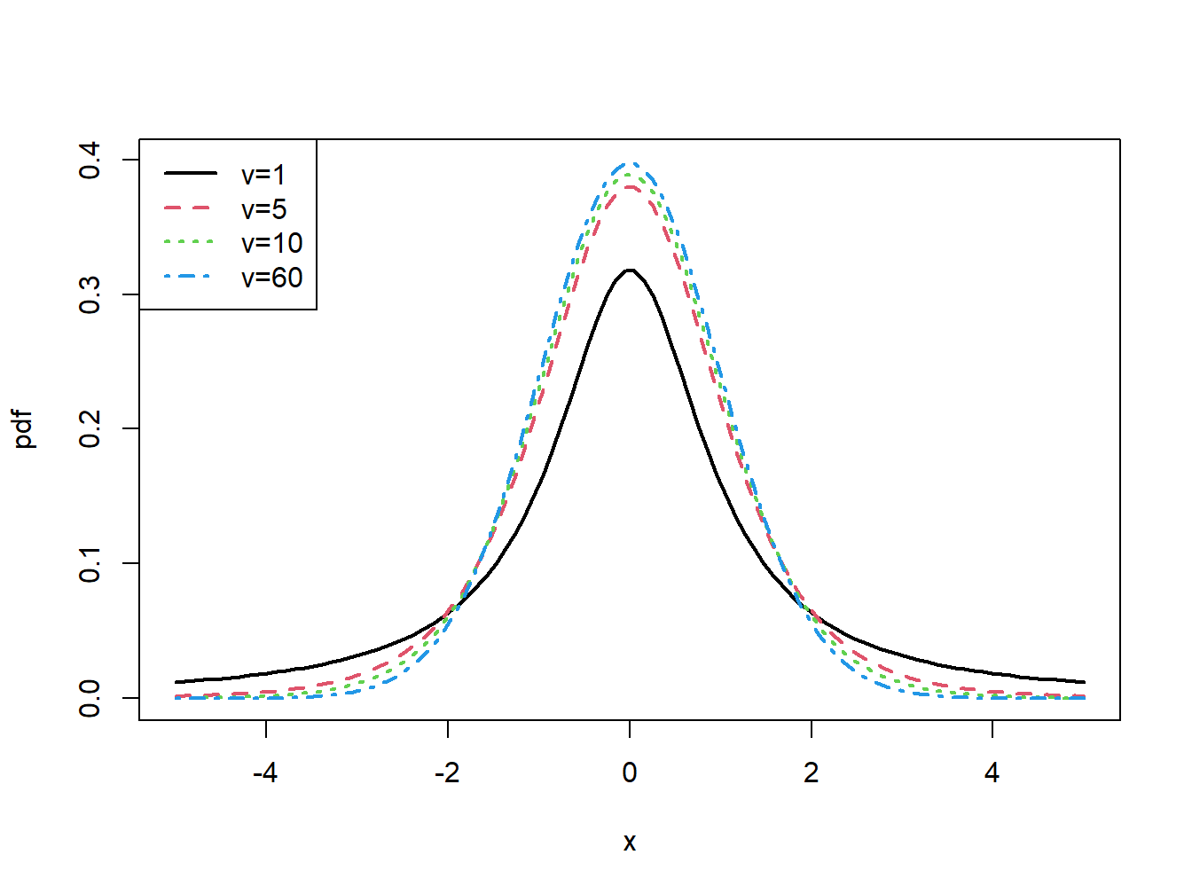
Figure 2.10: Student’s t density with \(v=1,5,10\) and \(60\).
The R functions pt() and qt() can be used to compute
the cdf and quantiles of a Student’s t random variable. For \(v=1,2,5,10,60,100\)
and \(\infty\) the 1% quantiles can be computed using:
## [1] -31.820516 -6.964557 -3.364930 -2.763769 -2.390119 -2.364217 -2.326348For \(v=1,2,5,10,60,100\) and \(\infty\) the values of \(\Pr(X<-3)\) are:
## [1] 0.102416382 0.047732983 0.015049624 0.006671828 0.001963849 0.001703958
## [7] 0.001349898
\(\blacksquare\)
2.1.7 Linear functions of a random variable
Let \(X\) be a random variable either discrete or continuous with \(E[X]=\mu_{X}\), \(\mathrm{var}(X)=\sigma_{X}^{2}\), and let \(a\) and \(b\) be known constants. Define a new random variable \(Y\) via the linear function of \(X\): \[ Y=g(X)=aX+b. \] Then the following results hold: \[\begin{align*} \mu_{Y} & =E[Y]=a\cdot E[X]+b=a\cdot\mu_{X}+b,\\ \sigma_{Y}^{2} & =\mathrm{var}(Y)=a^{2}\mathrm{var}(X)=a^{2}\sigma_{X}^{2},\\ \sigma_{Y} & =\mathrm{sd}(Y)=a\cdot\mathrm{sd}(X)=a\cdot\sigma_{X}. \end{align*}\] The first result shows that expectation is a linear operation. That is, \[ E[aX+b]=aE[X]+b. \] The second result shows that adding a constant to \(X\) does not affect its variance, and that the effect of multiplying \(X\) by the constant \(a\) increases the variance of \(X\) by the square of \(a.\) These results will be used often enough that it is instructive to go through the derivations.
Consider the first result. Let \(X\) be a discrete random variable. By the definition of \(E[g(X)]\), with \(g(X)=b+aX\), we have: \[\begin{align*} E[Y] & =\sum_{x\in S_{X}}(ax+b)\cdot\Pr(X=x)\\ & =a\sum_{x\in S_{X}}x\cdot\Pr(X=x)+b\sum_{x\in S_{X}}\Pr(X=x)\\ & =a\cdot E[X]+b\cdot1\\ & =a\cdot\mu_{X}+b. \end{align*}\] If \(X\) is a continuous random variable then by the linearity of integration: \[\begin{align*} E[Y] & =\int_{-\infty}^{\infty}(ax+b)f(x)~dx=a\int_{-\infty}^{\infty}xf(x)~dx+b\int_{-\infty}^{\infty}f(x)~dx\\ & =aE[X]+b. \end{align*}\] Next consider the second result. Since \(\mu_{Y}=a\mu_{X}+b\) we have: \[\begin{align*} \mathrm{var}(Y) & =E[(Y-\mu_{Y})^{2}]\\ & =E[(aX+b-(a\mu_{X}+b))^{2}]\\ & =E[(a(X-\mu_{X})+(b-b))^{2}]\\ & =E[a^{2}(X-\mu_{X})^{2}]\\ & =a^{2}E[(X-\mu_{X})^{2}]\textrm{ (by the linearity of }E[\cdot]\textrm{)}\\ & =a^{2}\mathrm{var}(X) \end{align*}\] Notice that the derivation of the second result works for discrete and continuous random variables.
A normal random variable has the special property that a linear function of it is also a normal random variable. The following proposition states the result.
Proposition 2.1 Let \(X\sim N(\mu_{X},\sigma_{X}^{2})\) and let \(a\) and \(b\) be constants. Let \(Y=aX+b\). Then \(Y\sim N(a\mu_{X}+b,a^{2}\sigma_{X}^{2})\).
The above property is special to the normal distribution and may or may not hold for a random variable with a distribution that is not normal.
Let \(X\) be a random variable with \(E[X]=\mu_{X}\) and \(\mathrm{var}(X)=\sigma_{X}^{2}\). Define a new random variable \(Z\) as: \[ Z=\frac{X-\mu_{X}}{\sigma_{X}}=\frac{1}{\sigma_{X}}X-\frac{\mu_{X}}{\sigma_{X}}, \] which is a linear function \(aX+b\) where \(a=\frac{1}{\sigma_{X}}\) and \(b=-\frac{\mu_{X}}{\sigma_{X}}\). This transformation is called standardizing the random variable \(X\) since, \[\begin{align*} E[Z] & =\frac{1}{\sigma_{X}}E[X]-\frac{\mu_{X}}{\sigma_{X}}=\frac{1}{\sigma_{X}}\mu_{X}-\frac{\mu_{X}}{\sigma_{X}}=0,\\ \mathrm{var}(Z) & =\left(\frac{1}{\sigma_{X}}\right)^{2}\mathrm{var}(X)=\frac{\sigma_{X}^{2}}{\sigma_{X}^{2}}=1. \end{align*}\] Hence, standardization creates a new random variable with mean zero and variance 1. In addition, if \(X\) is normally distributed then \(Z\sim N(0,1)\).
\(\blacksquare\)
Let \(X\sim N(2,4)\) and suppose we want to find \(\Pr(X>5)\) but we only know probabilities associated with a standard normal random variable \(Z\sim N(0,1)\). We solve the problem by standardizing \(X\) as follows: \[ \Pr\left(X>5\right)=\Pr\left(\frac{X-2}{\sqrt{4}}>\frac{5-2}{\sqrt{4}}\right)=\Pr\left(Z>\frac{3}{2}\right)=0.06681. \]
\(\blacksquare\)
Standardizing a random variable is often done in the construction of test statistics. For example, the so-called t-statistic or t-ratio used for testing simple hypotheses on coefficients is constructed by the standardization process.
A non-standard random variable \(X\) with mean \(\mu_{X}\) and variance \(\sigma_{X}^{2}\) can be created from a standard random variable via the linear transformation: \[\begin{equation} X=\mu_{X}+\sigma_{X}\cdot Z.\tag{2.23} \end{equation}\] This result is useful for modeling purposes as illustrated in the next examples.
Let \(X\sim N(\mu_{X},\sigma_{X}^{2})\). Quantiles of \(X\) can be conveniently computed using: \[\begin{equation} q_{\alpha}=\mu_{X}+\sigma_{X}z_{\alpha},\tag{2.24} \end{equation}\] where \(\alpha\in(0,1)\) and \(z_{\alpha}\) is the \(\alpha\times100\%\) quantile of a standard normal random variable. This formula is derived as follows. By the definition \(z_{\alpha}\) and (2.23) \[ \alpha=\Pr(Z\leq z_{\alpha})=\Pr\left(\mu_{X}+\sigma_{X}\cdot Z\leq\mu_{X}+\sigma_{X}\cdot z_{\alpha}\right)=\Pr(X\leq\mu_{X}+\sigma_{X}\cdot z_{\alpha}), \] which implies (2.24).
\(\blacksquare\)
The Student’s t distribution defined in (2.22) has zero mean and variance equal to \(v/(v-2)\) where \(v\) is the degrees of freedom parameter. We can define a Student’s t random variable with non-zero mean \(\mu\) and variance \(\sigma^{2}\) from a Student’s t random variable \(X\) as follows: \[ Y=\mu+\sigma\left(\frac{v-2}{v}\right)^{1/2}X=\mu+\sigma Z_{v}, \] where \(Z_{v}=\left(\frac{v-2}{v}\right)^{1/2}X\). The random variable \(Z_{v}\) is called a standardized Student’s t random variable with \(v\) degrees of freedom since \(E[Z_{v}]=0\) and \(\mathrm{var}(Z_{v})=\left(\frac{v-2}{v}\right)\mathrm{var}(X)=\left(\frac{v-2}{v}\right)\left(\frac{v}{v-2}\right)=1\). Then \[\begin{eqnarray*} E[Y] & = & \mu+\sigma E[Z]=\mu,\\ \mathrm{var}(Y) & = & \sigma^{2}\mathrm{var}(Z)=\sigma^{2}. \end{eqnarray*}\]
We use the notation \(Y \sim t_{v}(\mu, \sigma^{2})\) to denote that \(Y\) has a generalized Student’s t distribution with mean \(\mu\), variance \(\sigma^{2}\), and degrees of freedom \(v\).
\(\blacksquare\)
Let \(r\) denote the monthly continuously compounded return on an asset with \(E[r]=\mu\) and \(\mathrm{var}(R)=\sigma^{2}\). If \(r\) has a normal distribution or a general Student’s t distribution, then \(r\) can be expressed as: \[ r=\mu_{r}+\sigma_{r}\cdot\varepsilon, \] where \(\varepsilon \sim N(0,1)\) or \(\varepsilon \sim t_{v}(0,1)\). The random variable \(\varepsilon\) can be interpreted as representing the random news arriving in a given month that makes the observed return differ from its expected value \(\mu\). The fact that \(\varepsilon\) has mean zero means that news, on average, is neutral. The value of \(\sigma_{r}\) represents the typical size of a news shock. The bigger is \(\sigma_{r}\), the larger is the impact of a news shock and vice-versa. The distribution of \(\varepsilon\) impacts the likelihood of extreme new events (like stock market crashes). If \(\varepsilon \sim N(0,1)\) then extreme news events are not very likely. If \(\varepsilon \sim t_{v}(0,1)\) with \(v\) small (but bigger than 4) then extreme news events may happen from time-to-time.
\(\blacksquare\)
2.1.8 Value-at-Risk: An introduction
As an example of working with linear functions of a normal random variable, and to illustrate the concept of Value-at-Risk (VaR), consider an investment of $10,000 in Microsoft stock over the next month. Let \(R\) denote the monthly simple return on Microsoft stock and assume that \(R\sim N(0.05,(0.10)^{2})\). That is, \(E[R]=\mu_{R}=0.05\) and \(\mathrm{var}(R)=\sigma_{R}^{2}=(0.10)^{2}\). Let \(W_{0}\) denote the investment value at the beginning of the month and \(W_{1}\) denote the investment value at the end of the month. In this example, \(W_{0}=\$10,000\). Consider the following questions:
- What is the probability distribution of end-of-month wealth, \(W_{1}?\)
- What is the probability that end-of-month wealth is less than $9,000, and what must the return on Microsoft be for this to happen?
- What is the loss in dollars that would occur if the return on Microsoft stock is equal to its 5% quantile, \(q_{.05}\)? That is, what is the monthly 5% VaR on the $10,000 investment in Microsoft?
To answer (i), note that end-of-month wealth, \(W_{1}\), is related to initial wealth \(W_{0}\) and the return on Microsoft stock \(R\) via the linear function: \[ W_{1}=W_{0}(1+R)=W_{0}+W_{0}R=\$10,000+\$10,000\cdot R. \] Using the properties of linear functions of a random variable we have: \[ E[W_{1}]=W_{0}+W_{0}E[R]=\$10,000+\$10,000(0.05)=\$10,500, \] and, \[\begin{align*} \mathrm{var}(W_{1}) & =(W_{0})^{2}\mathrm{var}(R)=(\$10,000)^{2}(0.10)^{2},\\ \mathrm{sd}(W_{1}) & =(\$10,000)(0.10)=\$1,000. \end{align*}\] Further, since \(R\) is assumed to be normally distributed it follows that \(W_{1}\) is normally distributed: \[ W_{1}\sim N(\$10,500,(\$1,000)^{2}). \] To answer (ii), we use the above normal distribution for \(W_{1}\) to get: \[ \Pr(W_{1}<\$9,000)=0.067. \] To find the return that produces end-of-month wealth of $9,000, or a loss of $10,000-$9,000=$1,000, we solve \[ R=\frac{\$9,000-\$10,000}{\$10,000}=-0.10. \] If the monthly return on Microsoft is -10% or less, then end-of-month wealth will be $9,000 or less. Notice that \(R=-0.10\) is the 6.7% quantile of the distribution of \(R\): \[ \Pr(R<-0.10)=0.067. \] Question (iii) can be answered in two equivalent ways. First, we use \(R\sim N(0.05,(0.10)^{2})\) and solve for the 5% quantile of Microsoft Stock using (2.24)12: \[\begin{align*} \Pr(R & <q_{.05}^{R})=0.05\\ & \Rightarrow q_{.05}^{R}=\mu_{R}+\sigma_{R}\cdot z_{.05}=0.05+0.10\cdot(-1.645)=-0.114. \end{align*}\] That is, with 5% probability the return on Microsoft stock is -11.4% or less. Now, if the return on Microsoft stock is -11.4% the loss in investment value that occurs with 5% probability is \[ \mathrm{VaR}_{0.05} = W_{0}\cdot q_{.05}^{R} = \$10,000\cdot(0.114)= -\$1,144. \] Since losses are typically reported as positive numbers, \(\mathrm{VaR}_{0.05} = \$1,144\) is the 5% VaR over the next month on the $10,000 investment in Microsoft stock.
For the second method, use \(W_{1}\) ~ \(N(\$10,500,(\$1,000)^{2})\) and solve for the \(5\%\) quantile of end-of-month wealth directly: \[ \Pr(W_{1}<q_{.05}^{W_{1}})=0.05\Rightarrow q_{.05}^{W_{1}}=\$8,856. \] This corresponds to a loss of investment value of $10,000-$8,856=$1,144. Hence, if \(W_{0}\) represents the initial wealth and \(q_{.05}^{W_{1}}\) is the 5% quantile of the distribution of \(W_{1}\) then the 5% VaR is: \[ \textrm{ VaR}_{.05}=W_{0}-q_{.05}^{W_{1}}=\$10,000-\$8,856=\$1,144. \]
The following is the usual definition of VaR.Definition 2.14 If \(W_{0}\) represents the initial wealth in dollars and \(q_{\alpha}^{R}\) is the \(\alpha\times100\%\) quantile of distribution of the simple return \(R\) for small values of \(\alpha\), then the \(\alpha\times100\)% VaR is defined as: \[\begin{equation} \mathrm{VaR}_{\alpha}=-W_{0}\cdot q_{\alpha}^{R}.\tag{2.25} \end{equation}\]
In words, VaR\(_{\alpha}\) represents the dollar loss that could occur with probability \(\alpha\). By convention, it is reported as a positive number (hence the multiplication by minus one as \(q_{\alpha}^{R} < 0\) for small values of \(\alpha\)).
2.1.8.1 Value-at-Risk calculations for continuously compounded returns
The above calculations illustrate how to calculate VaR using the normal distribution for simple returns. However, as argued in Example 31, the normal distribution may not be appropriate for characterizing the distribution of simple returns and may be more appropriate for characterizing the distribution of continuously compounded returns. Let \(R\) denote the simple monthly return, let \(r=\ln(1+R)\) denote the continuously compounded return and assume that \(r\sim N(\mu_{r},\sigma_{r}^{2})\). The \(\alpha\times100\%\) monthly VaR on an investment of $\(W_{0}\) is computed using the following steps:
- Compute the \(\alpha\cdot100\%\) quantile, \(q_{\alpha}^{r}\), from the normal distribution for the continuously compounded return \(r\): \[ q_{\alpha}^{r}=\mu_{r}+\sigma_{r}z_{\alpha}, \] where \(z_{\alpha}\) is the \(\alpha\cdot100\%\) quantile of the standard normal distribution.
- Convert the continuously compounded return quantile, \(q_{\alpha}^{r}\), to a simple return quantile using the transformation: \[ q_{\alpha}^{R}=e^{q_{\alpha}^{r}}-1 \]
- Compute VaR using the simple return quantile (2.25).
Step 2 works because quantiles are preserved under monotonically increasing transformations of random variables.
Let \(R\) denote the simple monthly return on Microsoft stock and assume that \(R\sim N(0.05,(0.10)^{2})\). Consider an initial investment of \(W_{0}=\$10,000\). To compute the 1% and 5% VaR values over the next month use:
mu.R = 0.05
sd.R = 0.10
w0 = 10000
q.01.R = mu.R + sd.R*qnorm(0.01)
q.05.R = mu.R + sd.R*qnorm(0.05)
VaR.01 = -q.01.R*w0
VaR.05 = -q.05.R*w0
VaR.01
## [1] 1826.348## [1] 1144.854Hence with 1% and 5% probability the loss over the next month is at least $1,826 and $1,145, respectively.
Let \(r\) denote the continuously compounded return on Microsoft stock and assume that \(r\sim N(0.05,(0.10)^{2})\). To compute the 1% and 5% VaR values over the next month use:
mu.r = 0.05
sd.r = 0.10
q.01.R = exp(mu.r + sd.r*qnorm(0.01)) - 1
q.05.R = exp(mu.r + sd.r*qnorm(0.05)) - 1
VaR.01 = -q.01.R*w0
VaR.05 = -q.05.R*w0
VaR.01
## [1] 1669.277## [1] 1081.75Notice that when \(1+R=e^{r}\) has a log-normal distribution, the 1% and 5% VaR values (losses) are slightly smaller than when \(R\) is normally distributed. This is due to the positive skewness of the log-normal distribution.
\(\blacksquare\)
If \(P_{t+1}\) is a positive random variable such that \(\ln P_{t+1}\) is normally distributed then \(P_{t+1}\) has a log-normal distribution.↩︎
An inflection point is a point where a curve goes from concave up to concave down, or vice versa.↩︎
The inverse function of \(F_{X}\) , denoted \(F_{X}^{-1},\) has the property that \(F_{X}^{-1}(F_{X}(x))=x.\) \(F_{X}^{-1}\) will exist if \(F_{X}\) is strictly increasing and is continuous.↩︎
Using R, \(z_{.05}=\mathrm{qnorm}(0.05)=-1.645\).↩︎