13.5 Application to Vanguard Mutual Funds
In this section, we revisit the application of mean-variance portfolio theory to the problem of asset allocation among six Vanguard mutual funds that was discussed at the end of Chapter 12. For the sub-sample January, 2010 through December, 2014 it was shown that estimated mean-variance efficient portfolios had short sales in many of the Vanguard funds. Since it is not possible to short mutual funds, we re-estimate the efficient portfolios with the additional constraints that all portfolio weights must be positive. The monthly returns and annualized GWN model estimates for the Vanguard funds are created using:
data(VanguardPrices)
VanguardPrices = as.xts(VanguardPrices)
VanguardRetS = na.omit(Return.calculate(VanguardPrices, method="simple"))
smpl = "2010-1::2014-12"
r.f = 0.001
muhat = 12*colMeans(VanguardRetS[smpl])
covhat = 12*cov(VanguardRetS[smpl])
We use the IntroCompFinR portfolio functions to compute unrestricted and short-sales restricted estimates of the global minimum variance portfolio, the tangency portfolio, and the efficient frontier of risky assets:
# unrestricted (short sales allowed) portfolios
gmin.port = globalMin.portfolio(muhat, covhat)
tan.port = tangency.portfolio(muhat, covhat, r.f)
ef = efficient.frontier(muhat, covhat, alpha.min=0,
                        alpha.max=1.5, nport=20)
# short sales restricted portfolios
gmin.port.ns = globalMin.portfolio(muhat, covhat, shorts=FALSE)
tan.port.ns = tangency.portfolio(muhat, covhat, r.f, shorts=FALSE)
ef.ns = efficient.frontier(muhat, covhat, alpha.min=0,
                           alpha.max=1, nport=20, shorts=FALSE)
The global minimum variance portfolios are:
## Call:
## globalMin.portfolio(er = muhat, cov.mat = covhat)
##
## Portfolio expected return:     0.0197
## Portfolio standard deviation:  0.0114
## Portfolio weights:
##   vfinx   veurx   veiex   vbltx   vbisx   vpacx
## 0.0581 -0.0347 -0.0214 -0.0736 1.0647 0.0069## Call:
## globalMin.portfolio(er = muhat, cov.mat = covhat, shorts = FALSE)
##
## Portfolio expected return: 0.0218
## Portfolio standard deviation: 0.0135
## Portfolio weights:
## vfinx veurx veiex vbltx vbisx vpacx
## 0.0171 0.0000 0.0000 0.0000 0.9829 0.0000In the short sales restricted global minimum variance portfolio there is 98% weight on vbisx (low volatility US short-term bond fund) and 2% weight on vfinx (S&P 500 fund). The weights on other funds are pushed to zero. The volatility of the short sales restricted portfolio is slightly higher than the volatility of the unrestricted portfolio and so the cost of the short sales restrictions is small.
The estimated tangency portfolios are:
## Call:
## tangency.portfolio(er = muhat, cov.mat = covhat, risk.free = r.f)
##
## Portfolio expected return:     0.0642
## Portfolio standard deviation:  0.0209
## Portfolio Sharpe Ratio:        3.02
## Portfolio weights:
##   vfinx   veurx   veiex   vbltx   vbisx   vpacx
## 0.3152 -0.0907 -0.0874 0.1159 0.7387 0.0083## Call:
## tangency.portfolio(er = muhat, cov.mat = covhat, risk.free = r.f,
## shorts = FALSE)
##
## Portfolio expected return: 0.0637
## Portfolio standard deviation: 0.0287
## Portfolio Sharpe Ratio: 2.18
## Portfolio weights:
## vfinx veurx veiex vbltx vbisx vpacx
## 0.192 0.000 0.000 0.245 0.563 0.000The short sales restricted tangency portfolio has positive weights on vfinx, vbltx, and vbisx and zero weights for the remaining assets. The Sharpe ratio of the short sales restricted tangency portfolio, however, is substantially smaller than the Sharpe ratio of the unrestricted portfolio.
Figure 13.11 shows the short sales restricted and unrestricted efficient portfolio frontiers, created using:
# unrestricted efficient frontiers
plot(ef, plot.assets=TRUE, col="blue", pch=16)
text(tan.port$sd, tan.port$er,labels = "tan", pos = 2)
sr.tan = (tan.port$er - r.f)/tan.port$sd
text(0, r.f, labels=expression(r[f]), pos = 4)
abline(a=r.f, b=sr.tan, col="green", lwd=2)
abline(h=0, v=0)
# short sales restricted frontiers
sr.tan.ns = (tan.port.ns$er - r.f)/tan.port.ns$sd
points(ef.ns$sd, ef.ns$er, type="b", pch=16, col="red")
abline(a=r.f, b=sr.tan.ns, col="green", lwd=2)
text(tan.port.ns$sd, tan.port.ns$er,labels = "tan (no shorts)", pos = 4)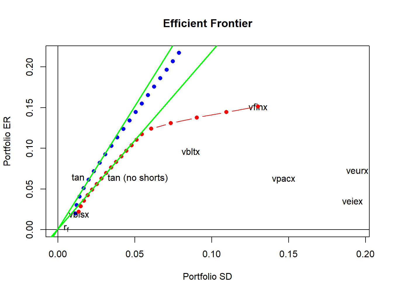
Figure 13.11: Unrestricted and short sales restricted efficient portfolio frontiers.
The short sales restricted risky asset only frontier, shown in red, lies underneath and to the right of the unrestricted risky asset frontier, shown in blue. The short sales restricted tangency portfolio has a similar expected return as the unrestricted tangency portfolio but has a higher volatility and a lower Sharpe ratio.