4.2 Multivariate Time Series

Consider $n$ time series variables $\{Y_{1t}\},\ldots,\{Y_{nt}\}$. A multivariate time series is the $(n\times1)$ vector time series $\{\mathbf{Y}_{t}\}$ where the $i^{th}$ row of $\{\mathbf{Y}_{t}\}$ is $\{Y_{it}\}$. That is, for any time $t$, $\mathbf{Y}_{t}=(Y_{1t},\ldots,Y_{nt})^{\prime}$. Multivariate time series analysis is used when one wants to model and explain the interactions and co-movements among a group of time series variables. In finance, multivariate time series analysis is used to model systems of asset returns, asset prices, exchange rates, the term structure of interest rates, and economic variables, etc.. Many of the time series concepts described previously for univariate time series carry over to multivariate time series in a natural way. Additionally, there are some important time series concepts that are particular to multivariate time series. The following sections give the details of these extensions.

4.2.1 Stationary and ergodic multivariate time series

A multivariate time series $\{\mathbf{Y}_{t}\}$ is covariance stationary and ergodic if all of its component time series are stationary and ergodic. The mean of $\mathbf{Y}_{t}$ is defined as the $(n\times1)$ vector $$E[\mathbf{Y}_{t}]=(\mu_{1},\ldots,\mu_{n})^{\prime}=\mu,$$ where $\mu_{i}=E[Y_{it}]$ for $i=1,\ldots,n$. The variance/covariance matrix of $\mathbf{Y}_{t}$ is the $(n\times n)$ matrix $$\begin{align*} \mathrm{var}(\mathbf{Y}_{t}) & =\Sigma=E[(\mathbf{Y}_{t}-\mu)(\mathbf{Y}_{t}-\mu)^{\prime}]\\ & =\left(\begin{array}{cccc} \mathrm{var}(Y_{1t}) & \mathrm{cov}(Y_{1t},Y_{2t}) & \cdots & \mathrm{cov}(Y_{1t},Y_{nt})\\ \mathrm{cov}(Y_{2t},Y_{1t}) & \mathrm{var}(Y_{2t}) & \cdots & \mathrm{cov}(Y_{2t},Y_{nt})\\ \vdots & \vdots & \ddots & \vdots\\ \mathrm{cov}(Y_{nt},Y_{1t}) & \mathrm{cov}(Y_{nt},Y_{2t}) & \cdots & \mathrm{var}(Y_{nt}) \end{array}\right). \end{align*}$$ The matrix $\Sigma$ has elements $\sigma_{ij}=$ cov$(Y_{it},Y_{jt})$ which measure the contemporaneous linear dependence between $Y_{it}$ and $Y_{jt}$ that is time invariant. The correlation matrix of $\mathbf{Y}_{t}$ is the $(n\times n)$ matrix $$\mathrm{cor}(\mathbf{Y}_{t})=\mathbf{C}_{0}=\mathbf{D}^{-1} \Gamma_{0} \mathbf{D}^{-1},$$ where $\mathbf{D}$ is an $(n\times n)$ diagonal matrix with $j^{th}$ diagonal element $\sigma_{j}=\mathrm{sd}(Y_{jt})$.

4.2.1.1 Cross covariance and correlation matrices

For a univariate time series $\{Y_{t}\}$, the autocovariances, $\gamma_{k}$, and autocorrelations, $\rho_{k}$, summarize the linear time dependence in the data. With a multivariate time series $\{\mathbf{Y}_{t}\}$ each component has autocovariances and autocorrelations but there are also cross lead-lag covariances and correlations between all possible pairs of components. The lag $k$ autocovariances and autocorrelations of $Y_{jt}$, for $j=1,\ldots,n$, are defined as $$\begin{align*} \gamma_{jj}^{k} & =\mathrm{cov}(Y_{jt},Y_{jt-k}),\\ \rho_{jj}^{k} & =\mathrm{corr}(Y_{jt},Y_{jt-k})=\frac{\gamma_{jj}^{k}}{\sigma_{j}^{2}}, \end{align*}$$ and these are symmetric in $k$: $\gamma_{jj}^{k}=\gamma_{jj}^{-k}$, $\rho_{jj}^{k}=\rho_{jj}^{-k}$. The cross lag-k covariances and cross lag-k correlations between $Y_{it}$ and $Y_{jt}$ are defined as $$\begin{align*} \gamma_{ij}^{k} & =\mathrm{cov}(Y_{it},Y_{jt-k}),\\ \rho_{ij}^{k} & =\mathrm{corr}(Y_{jt},Y_{jt-k})=\frac{\gamma_{ij}^{k}}{\sqrt{\sigma_{i}^{2}\sigma_{j}^{2}}}, \end{align*}$$ and they are not necessarily symmetric in $k$. In general, $$\gamma_{ij}^{k}=\mathrm{cov}(Y_{it},Y_{jt-k})\neq\mathrm{cov}(Y_{jt},Y_{it-k})=\gamma_{ji}^{k}.$$ If $\gamma_{ij}^{k}\neq0$ for some $k>0$ then $Y_{jt}$ is said to lead $Y_{it}$. This implies that past values of $Y_{jt}$ are useful for predicting future values of $Y_{it}.$ Similarly, if $\gamma_{ji}^{k}\neq0$ for some $k>0$ then $Y_{it}$ is said to lead $Y_{jt}$. It is possible that $Y_{it}$ leads $Y_{jt}$ and vice-versa. In this case, there is said to be dynamic feedback between the two series.

All of the lag $k$ cross covariances and correlations are summarized in the $(n\times n)$ lag $k$ cross covariance and lag $k$ cross correlation matrices $$\begin{align*} \mathbf{\Gamma}_{k} & =E[(\mathbf{Y}_{t}-\mathbf{\mu)(Y}_{t-k}-\mu)^{\prime}]\\ & =\left(\begin{array}{cccc} \mathrm{cov}(Y_{1t},Y_{1t-k}) & \mathrm{cov}(Y_{1t},Y_{2t-k}) & \cdots & \mathrm{cov}(Y_{1t},Y_{nt-k})\\ \mathrm{cov}(Y_{2t},Y_{1t-k}) & \mathrm{cov}(Y_{2t},Y_{2t-k}) & \cdots & \mathrm{cov}(Y_{2t},Y_{nt-k})\\ \vdots & \vdots & \ddots & \vdots\\ \mathrm{cov}(Y_{nt},Y_{1t-k}) & \mathrm{cov}(Y_{nt},Y_{2t-k}) & \cdots & \mathrm{cov}(Y_{nt},Y_{nt-k}) \end{array}\right),\\ \mathbf{C}_{k} & \mathbf{=}\mathbf{D}^{-1}\mathbf{\Gamma}_{k}\mathbf{D}^{-1}. \end{align*}$$ The matrices $\mathbf{\Gamma}_{k}$ and $\mathbf{C}_{k}$ are not symmetric in $k$ but it is easy to show that $\mathbf{\Gamma}_{-k}=\mathbf{\Gamma}_{k}^{\prime}$ and $\mathbf{C}_{-k}=\mathbf{C}_{k}^{\prime}$.

Example 4.5 (Multivariate Gaussian white noise processes)

Let $\{\mathbf{Y}_{t}\}$ be an $n\times1$ vector time series process. If $\mathbf{Y}_{t}\sim iid\,N(\mathbf{0},\,\Sigma)$ then $\{\mathbf{Y}_{t}\}$ is called multivariate Gaussian white noise and is denoted $\mathbf{Y}_{t}\sim\mathrm{GWN}(\mathbf{0},\,\Sigma)$. Notice that $$\begin{eqnarray*} E[\mathbf{Y}_{t}] & = & \mathbf{0},\\ \mathrm{var}(\mathbf{Y}_{t}) & = & \Sigma,\\ \mathrm{cov}(Y_{jt},Y_{jt-k}) & = & \gamma_{jj}^{k}=0\,(\textrm{for}\,k>0)\\ \mathrm{cov}(Y_{it},Y_{jt-k}) & = & \gamma_{ij}^{k}=0\,(\textrm{for}\,k>0) \end{eqnarray*}$$ Hence, the elements of $\{\mathbf{Y}_{t}\}$ are contemporaneously correlated but exhibit no time dependence. That is, each element of $\mathbf{Y}_{t}$ exhibits no time dependence and there is no dynamic feedback between any two elements. Simulating observations from $\mathrm{GWN}(\mathbf{0},\,\Sigma)$ requires simulating from a multivariate normal distribution, which can be done using the mvtnorm function rmvnorm(). For example, to simulate and plot $T=250$ observation from a bivariate $\mathrm{GWN}(\mathbf{0},\,\Sigma)$ process with $$\Sigma=\left(\begin{array}{cc} 4 & 1\\ 1 & 1 \end{array}\right)\Rightarrow C=\left(\begin{array}{cc} 1 & 0.5\\ 0.5 & 1 \end{array}\right)$$ use:

library(mvtnorm) 
Sigma = matrix(c(4, 1, 1, 1), 2, 2) 
set.seed(123) 
Y = rmvnorm(250, sigma=Sigma) 
colnames(Y) = c("Y1", "Y2") 
ts.plot(Y, lwd=2, col=c("black", "blue")) 
abline(h=0)
legend("topleft", legend=c("Y1", "Y2"), 
       lwd=2, col=c("black", "blue"), lty=1)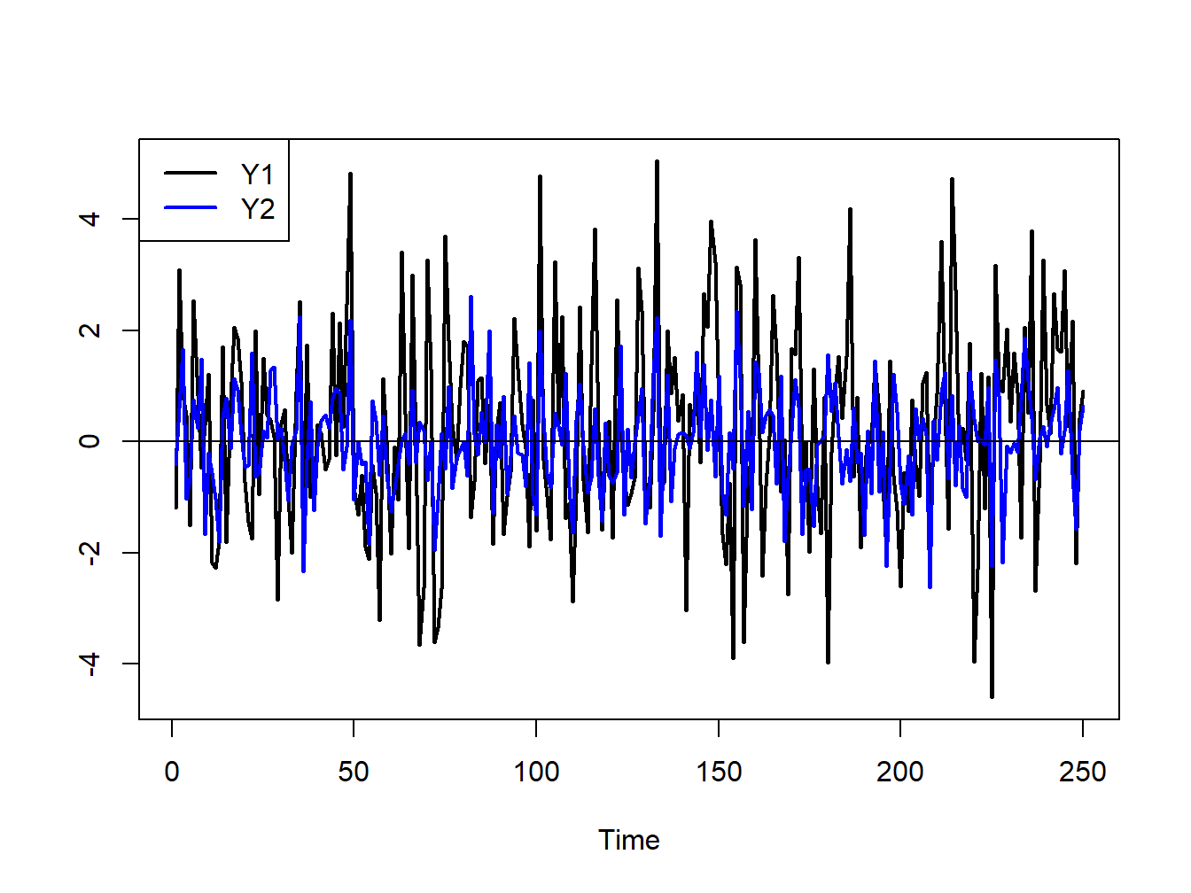

Figure 4.7: Simulated bivariate GWN process.

The simulated values are shown on the same plot in Figure 4.7. Both series fluctuate randomly about zero, and the first series (black line) has larger fluctuations (volatility) than the second series (blue line). The two series are contemporaneously correlated $(\rho_{12}=0.5)$ but are both uncorrelated over time ($\rho_{11}^{k}=\rho_{22}^{k}=0,\,k>0)$ and are not cross-lag correlated ($\rho_{12}^{k}=\rho_{21}^{k}=0,\,k>0$).

$\blacksquare$