6.2 Monte Carlo Simulation of the GWN Model

A simple technique that can be used to understand the probabilistic behavior of a model involves using computer simulation methods to create pseudo data from the model. The process of creating such pseudo data is called Monte Carlo simulation.³² Monte Carlo simulation of a model can be used as a first step reality check of the model. If simulated data from the model do not look like the data that the model is supposed to describe, then serious doubt is cast on the model. However, if simulated data look reasonably close to the actual data then the first step reality check is passed. Ideally, one should consider many simulated samples from the model because it is possible for a given simulated sample to look strange simply because of an unusual set of random numbers.

Monte Carlo simulations can be used to reveal properties of a model that are hard to derive analytically.

Monte Carlo simulation can also be used to create “what if?” type scenarios for a model. Different scenarios typically correspond with different model parameter values.

Finally, Monte Carlo simulation can be used to study properties of statistics computed from the pseudo data from the model. For example, Monte Carlo simulation can be used to illustrate the concepts of estimator bias and confidence interval coverage probabilities (see Chapter 9).

To illustrate the use of Monte Carlo simulation, consider creating pseudo return data from the GWN model (6.1) for a single asset. The steps to create a Monte Carlo simulation from the GWN model are:

Monte Carlo Steps: Single Asset

Fix values for the GWN model parameters $\mu$ and $\sigma$.
Determine the number of simulated values, $T$, to create.
Use a computer random number generator to simulate $T$ $iid$ values of $\varepsilon_{t}$ from a $N(0,\sigma^{2})$ distribution. Denote these simulated values as $\tilde{\varepsilon}_{1},\ldots,\tilde{\varepsilon}_{T}$.
Create the simulated return data $\tilde{R}_{t}=\mu+\tilde{\varepsilon}_{t}$ for $t=1,\ldots,T$.

Example 2.3 (Microsoft data to calibrate univariate Monte Carlo simulation of GWN model)

To motivate plausible values for $\mu$ and $\sigma$ in the simulation, Figure 6.1 shows the monthly continuously compounded (cc) returns on Microsoft stock over the period January 1998 through May 2012. The data is the same as that used in Chapter 5 and is constructed from the IntroCompFinR "xts" object msftDailyPrices as follows:

data(msftDailyPrices) 
msftPrices = to.monthly(msftDailyPrices, OHLC=FALSE) 
smpl = "1998-01::2012-05" 
msftPrices = msftPrices[smpl] 
msftRetC = na.omit(Return.calculate(msftPrices, method="log"))
mu.msftRetC = mean(msftRetC)
sigma.msftRetC = sd(msftRetC)
c(mu.msftRetC, sigma.msftRetC)

## [1] 0.004125523 0.100212624

The parameter $\mu=E[R_{t}]$ in the GWN model is the expected monthly return, and $\sigma$ represents the typical size of a deviation about $\mu$. In Figure 6.1, the returns seem to fluctuate up and down about a central value near 0 and the typical size of a return deviation about 0 is roughly 0.10, or 10% (see dashed lines in Figure 6.1). The sample mean turns out to be $\hat{\mu}=0.004$ (0.4%) and the sample standard deviation is $\hat{\sigma}=0.100$ (10%). Figure 6.2 shows three distribution summaries (histogram, boxplot and normal qq-plot) and the SACF computed from the sample returns. The returns look to have slightly fatter tails than the normal distribution and show little evidence of linear time dependence (autocorrelation).

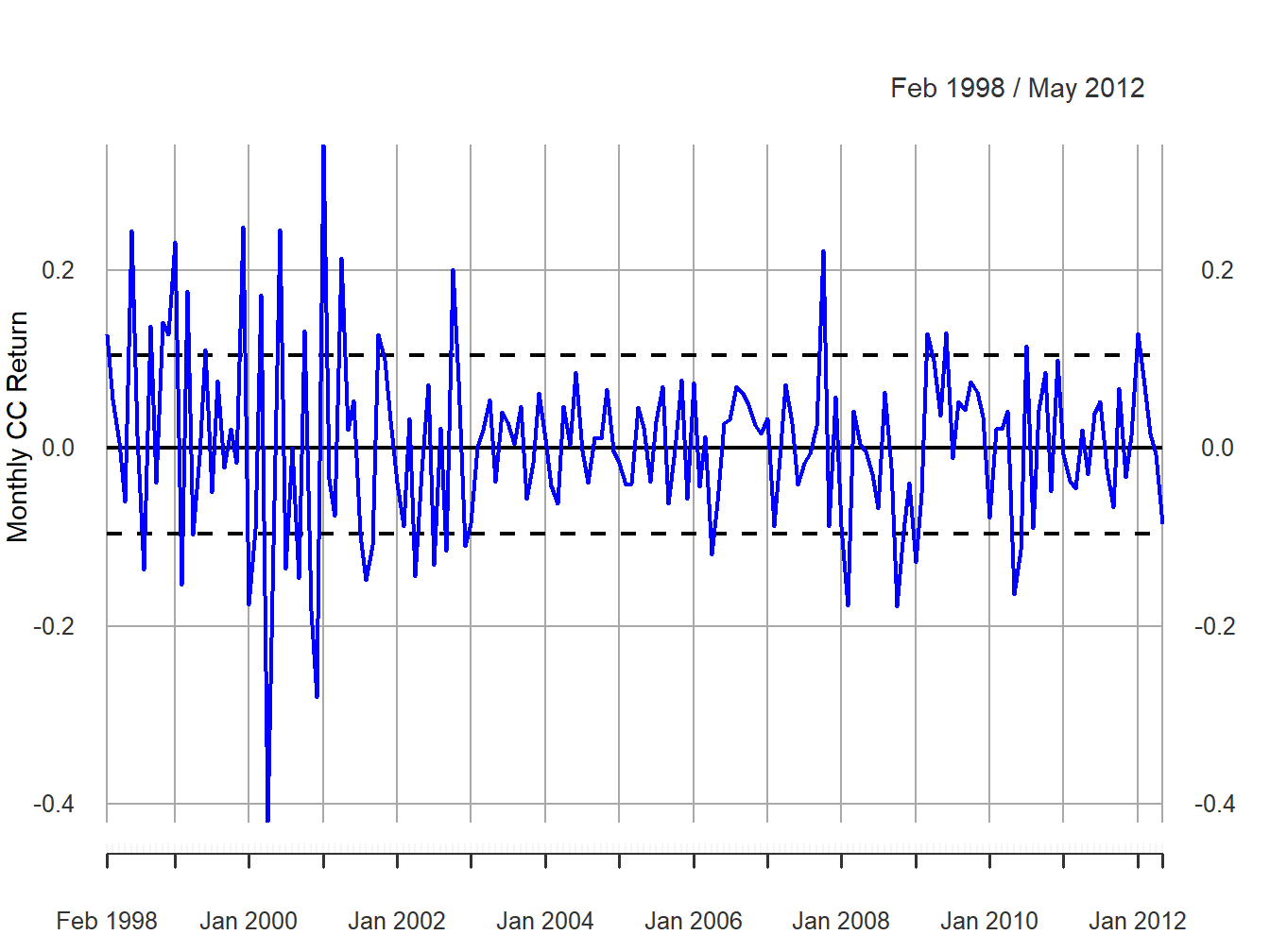
$Monthly cc returns on Microsoft. Dashed lines indicate $\hat{\mu}\pm\hat{\sigma}$.$

Figure 6.1: Monthly cc returns on Microsoft. Dashed lines indicate $\hat{\mu}\pm\hat{\sigma}$.

$\blacksquare$

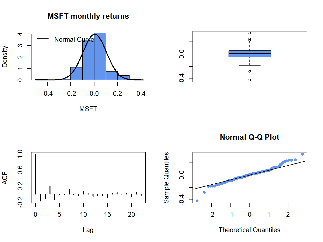
Figure 6.2: Graphical descriptive statistics for the monthly cc returns on Microsoft.

Example 4.2 (Simulating observations from the GWN model)

To mimic the monthly return data on Microsoft in the Monte Carlo simulation, the values $\mu=0.004$ and $\sigma=0.10$ are used as the model’s true parameters and $T=172$ is the number of simulated values (sample size of actual data). Let $\{\tilde{\varepsilon}_{1},\ldots,\tilde{\varepsilon}_{172}\}$ denote the $172$ simulated values of the random news variable $\varepsilon_{t}\sim\mathrm{GWN}(0,(0.10)^{2})$. The simulated returns are then computed using:³³ \[\begin{equation} \tilde{R}_{t}=0.004+\tilde{\varepsilon}_{t},~t=1,\ldots,172\tag{6.8} \end{equation}\] To create the simulated returns from (6.8) use:

mu = 0.004
sd.e = 0.10
n.obs = length(msftRetC)
set.seed(111)
sim.e = rnorm(n.obs, mean=0, sd=sd.e)
sim.ret = mu + sim.e
sim.ret = xts(sim.ret, index(msftRetC))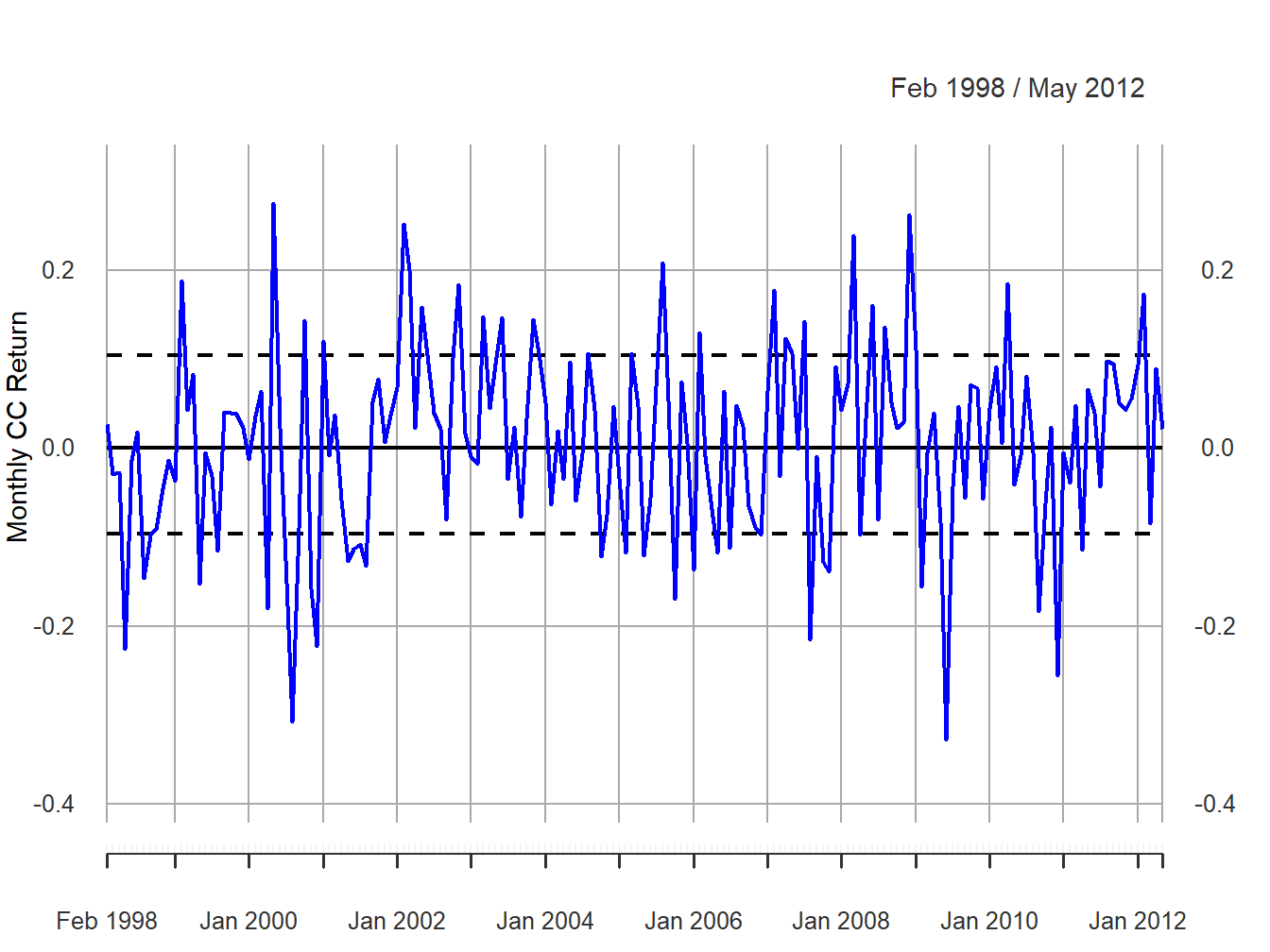

Figure 6.3: Monte Carlo simulated cc returns from the GWN model for Microsoft.

The simulated returns $\{\tilde{R}_{t}\}_{t=1}^{172}$ (with the same time index as the Microsoft returns) are shown in Figure 6.3. The simulated return data fluctuate randomly about $\mu=0.004$, and the typical size of the fluctuation is approximately equal to $\sigma=0.10$. The simulated return data look somewhat like the actual monthly return data for Microsoft. The main difference is that the return volatility for Microsoft appears to have decreased in the latter part of the sample whereas the simulated data has constant volatility over the entire sample. Figure 6.4 shows the distribution summaries (histogram, boxplot and normal qq-plot) and the SACF for the simulated returns. The simulated returns are normally distributed and show thinner tails than the actual returns. The simulated returns also show no evidence of linear time dependence (autocorrelation).

$\blacksquare$

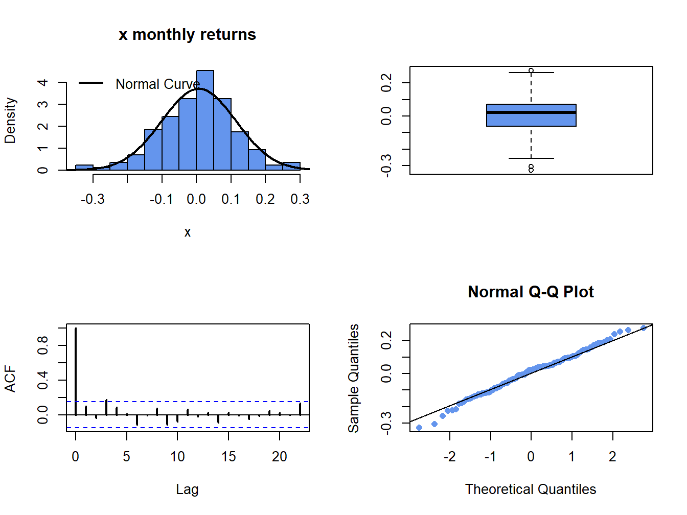
Figure 6.4: Graphical descriptive statistics for the Monte Carlo simulated returns on Microsoft.

Example 4.3 (Simulating log-prices and prices from the RW model)

The RW model for log-price based on the GWN model (6.8) calibrated to Microsoft log prices is: \[ p_{t}=2.592+0.004\cdot t+\sum_{j=1}^{t}\varepsilon_{j},\varepsilon_{j}\sim\mathrm{GWN}(0,(0.10)^{2}). \] where $p_{0}=2.586=\ln(13.27)$ is the log of Microsoft Price at the end of January 1998. Given $p_{t}$, the price level is determined using $P_{t} = e^{p_{t}}$. A Monte Carlo simulation of this RW model with drift can be created in R using:

p0 = 2.58
sim.p = p0 + mu*seq(n.obs) + cumsum(sim.e)
sim.p = c(p0, sim.p)
sim.P = exp(sim.p)
sim.p = xts(sim.p, index(msftPrices)) 
sim.P = xts(sim.P, index(msftPrices))

Figure 6.5 shows the simulated log prices and prices. The top panel shows the simulated log price, $\tilde{p}_{t}$, and the bottom panel shows the simulated price levels $\tilde{P}_{t}=e^{\tilde{p}_{t}}$ For comparison, Figure 6.6 shows the actual log prices and price levels for Microsoft stock. Notice the similar behavior of the simulated random walk data and the actual data.

$\blacksquare$

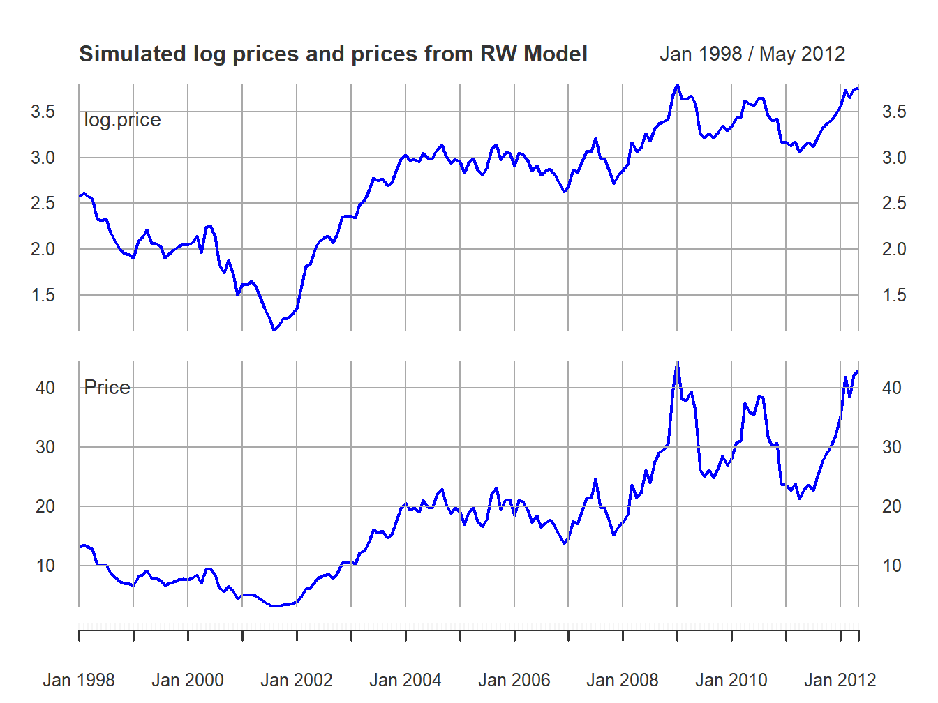
Top panel: Simulated log monthly prices of Microsoft from RW model. Bottom panel: Simulated monthly prices of Micorosft stock from RW model.

Figure 6.5: Top panel: Simulated log monthly prices of Microsoft from RW model. Bottom panel: Simulated monthly prices of Micorosft stock from RW model.

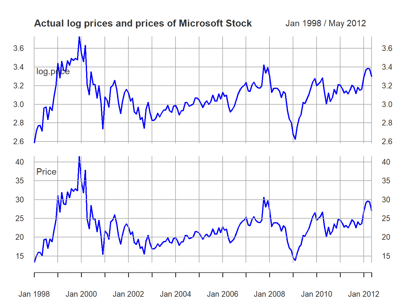
Figure 6.6: Top panel: Actual log monthly prices of Microsoft. Bottom panel: Actual monthly prices of Microsoft stock.

The previous examples show one Monte Carlo simulation from the GWN model for cc returns. The simulated returns were compared to the actual returns to do the first stage reality check. Here, the simulated returns looked similar to actual returns so the GWN model passed the first stage reality check. However, keep in mind that the simulated returns represent only one random draw of size $T$ from the GWN model for cc returns. It is possible that you can, by chance, get a strange set of simulated returns which would lead you to reject the first stage reality check even if the GWN model is a good model for actual returns. To guard against this possibility, you should always create many Monte Carlo simulations from the proposed model and use the typical behavior from the simulations to do the first step reality check.

Example 2.5 (Creating many simulations from the GWN model)

To create ten simulated samples of size $T=132$ from the GWN model for Microsoft cc returns use:

sim.e = matrix(0, n.obs, 10)
set.seed(111)
for (i in 1:10) {
sim.e[,i] = rnorm(n.obs, mean=0, sd=sd.e)
}
sim.ret = mu + sim.e
sim.ret = xts(sim.ret, index(msftRetC))
colnames(sim.ret) = paste("sim", 1:10, sep=".")

The ten simulations are shown in Figure 6.7.

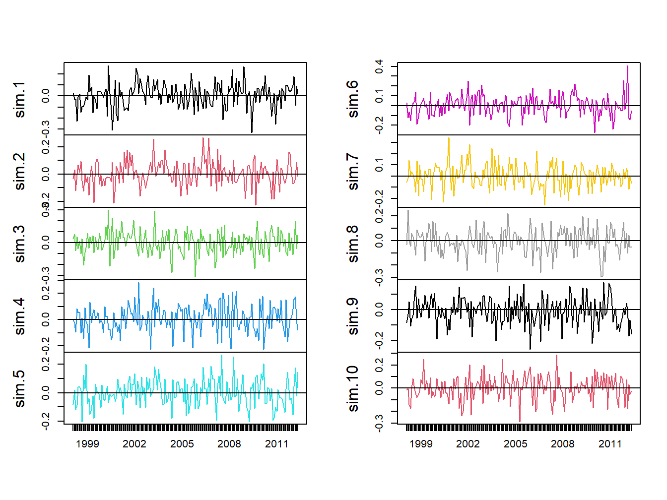
Figure 6.7: Ten Simulations from GWN Model for Microsoft CC Returns.

Each panel shows an alternative reality for returns over the period February 1998 through May 2012. Each one of these alternative realities is equally likely to happen, and the typical behavior of the simulated returns is similar to actual returns.

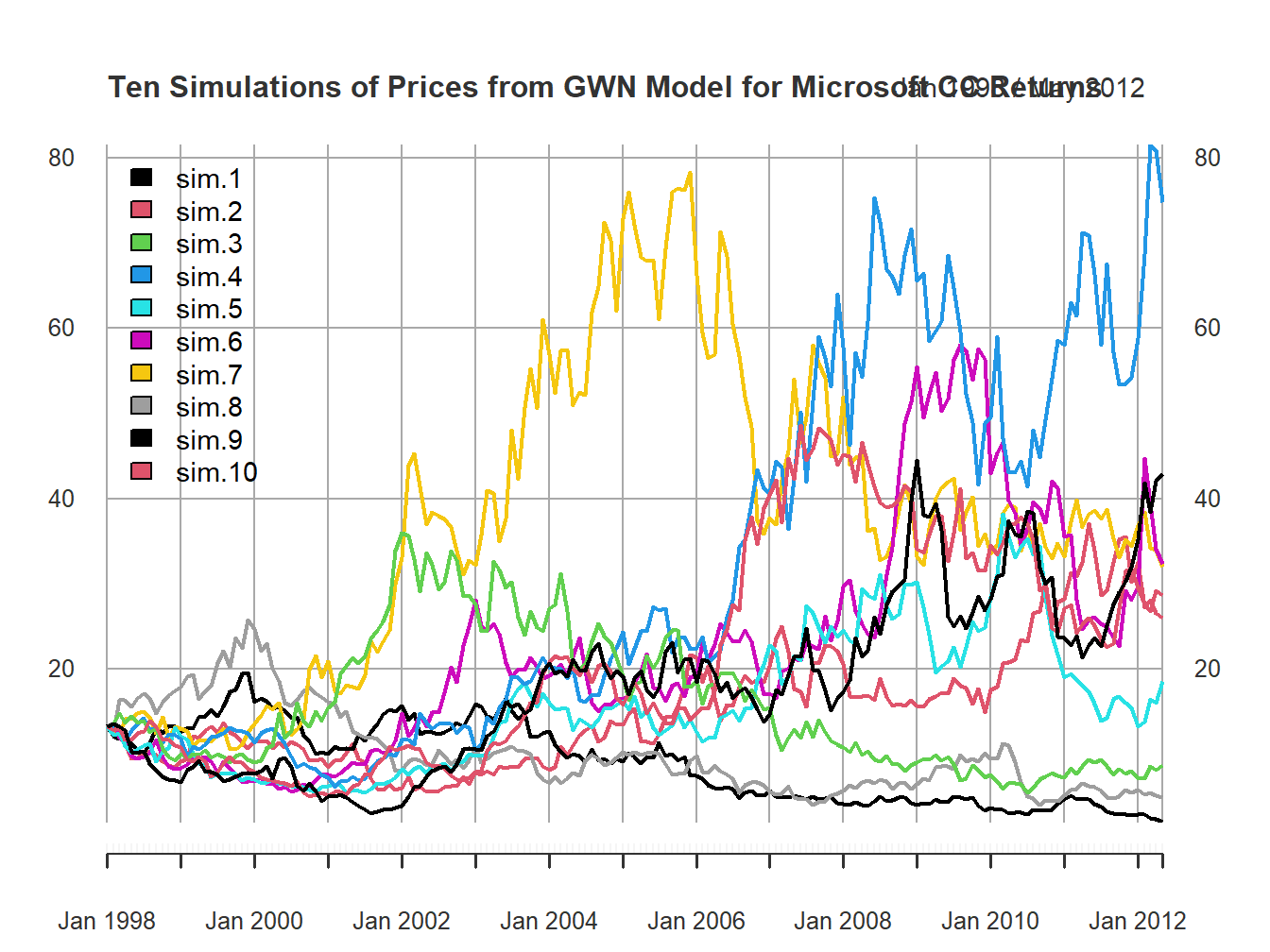
Figure 6.8: Ten Price Simulations from GWN Model for Microsoft CC Returns.

Figure 6.8 shows the same ten simulations from the GWN model in terms of prices. Notice the large variability in prices at the end of the sample.

6.2.1 Simulating returns on more than one asset

Creating a Monte Carlo simulation of more than one return from the GWN model requires simulating observations from a multivariate normal distribution. This follows from the matrix representation of the GWN model given in (6.3). The steps required to create a multivariate Monte Carlo simulation are:

Monte Carlo Steps: Multiple Assets

Fix values for the $N\times 1$ mean vector $\mu$ and the $N\times N$ covariance matrix $\Sigma$.
Determine the number of simulated values, $T,$ to create.
Use a computer random number generator to simulate $T$ $iid$ values of the $N\times 1$ random vector $\varepsilon_{t}$ from the multivariate normal distribution $N(\mathbf{0},\Sigma)$. Denote these simulated vectors as $\tilde{\varepsilon}_{1},\ldots,\tilde{\varepsilon}_{T}$.
Create the $N\times 1$ simulated return vector $\mathbf{\tilde{R}}_{t}=\mu+\tilde{\varepsilon}_{t}$ for $t=1,\ldots,T$.
Repeat steps 1-4 to create multiple simulations (alternative realities).

Example 2.6 (Microsoft, Starbucks and S&P 500 data to calibrate multivariate Monte Carlo simulation of GWN model)

To motivate the parameters for a multivariate simulation of the GWN model, consider the monthly cc returns for Microsoft, Starbucks and the S&P 500 index over the period January 1998 through May 2012 illustrated in Figures 6.9 and 6.10. The data is assembled using the R commands:

data(sp500DailyPrices, sbuxDailyPrices) 
sp500Prices = to.monthly(sp500DailyPrices, OHLC=FALSE) 
sbuxPrices = to.monthly(sbuxDailyPrices, OHLC=FALSE) 
sp500Prices = sp500Prices[smpl] 
sbuxPrices = sbuxPrices[smpl] 
sp500RetC = na.omit(Return.calculate(sp500Prices, method="log"))
sbuxRetC = na.omit(Return.calculate(sbuxPrices, method="log"))
gwnRetC = merge(msftRetC, sbuxRetC, sp500RetC) 
colnames(gwnRetC) = c("MSFT", "SBUX", "SP500")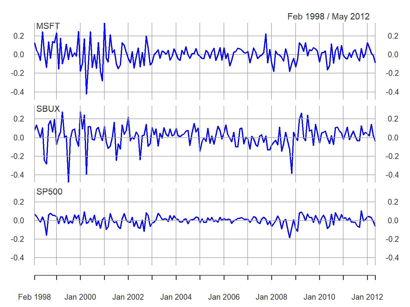

$Monthly cc returns on Microsoft, Starbucks, and the S\&P 500 Index.$

Figure 6.9: Monthly cc returns on Microsoft, Starbucks, and the S&P 500 Index.

The multivariate sample descriptive statistics (mean vector, standard deviation vector, covariance matrix and correlation matrix) are:

mean.vals = apply(gwnRetC, 2, mean)
sd.vals = apply(gwnRetC, 2, sd)
rbind(mean.vals, sd.vals)

##                  MSFT       SBUX       SP500
## mean.vals 0.004125523 0.01465698 0.001687186
## sd.vals   0.100212624 0.11164481 0.048470624

cov(gwnRetC)

##              MSFT        SBUX       SP500
## MSFT  0.010042570 0.003814041 0.002997879
## SBUX  0.003814041 0.012464565 0.002475527
## SP500 0.002997879 0.002475527 0.002349401

cor(gwnRetC)

##            MSFT      SBUX     SP500
## MSFT  1.0000000 0.3408979 0.6171816
## SBUX  0.3408979 1.0000000 0.4574573
## SP500 0.6171816 0.4574573 1.0000000

All returns fluctuate around mean values close to zero. The volatilities of Microsoft and Starbucks are similar with typical magnitudes around 0.10, or 10%. The volatility of the S&P 500 index is considerably smaller at about 0.05, or 5%. The pairwise scatterplots show that all returns are positively related. The pairs (MSFT, SP500) and (SBUX, SP500) are the most correlated with sample correlation values around 0.5. The pair (MSFT, SBUX) has a moderate positive correlation around 0.3.

$\blacksquare$

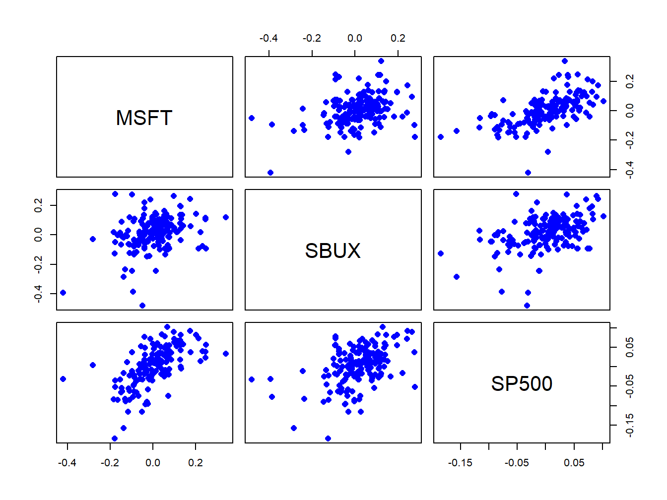
$Pairwise scatterplots of the monthly returns on Microsoft, Starbucks, and the S\&P 500 Index.$

Figure 6.10: Pairwise scatterplots of the monthly returns on Microsoft, Starbucks, and the S&P 500 Index.

Example 4.4 (Monte Carlo simulation of GWN model for three assets)

Simulating values from the multivariate GWN model (6.3) requires simulating multivariate normal random variables. In R, this can be done using the function rmvnorm() from the package mvtnorm. The function rmvnorm() requires a vector of mean values and a covariance matrix. Define: \[ \mathbf{R}_{t}=\left(\begin{array}{c} R_{\textrm{msft},t}\\ R_{\textrm{sbux},t}\\ R_{\textrm{sp500},t} \end{array}\right),~\mu=\left(\begin{array}{c} \mu_{\textrm{msft},t}\\ \mu_{\textrm{sbux},t}\\ \mu_{\textrm{sp500},t} \end{array}\right),\Sigma=\left(\begin{array}{ccc} \sigma_{\textrm{msft}}^{2} & \sigma_{\textrm{msft},\textrm{sbux}} & \sigma_{\textrm{msft},\textrm{sp500}}\\ \sigma_{\textrm{msft},\textrm{sbux}} & \sigma_{\textrm{sbux}}^{2} & \sigma_{\textrm{sbux},\textrm{sp500}}\\ \sigma_{\textrm{msft},\textrm{sp500}} & \sigma_{\textrm{sbux},\textrm{sp500}} & \sigma_{\textrm{sp500}}^{2} \end{array}\right) \] The parameters $\mu$ and $\Sigma$ of the multivariate GWN model are set equal to the sample mean vector $\mu$ and sample covariance matrix $\Sigma$:

muVec = apply(gwnRetC, 2, mean)
covMat = cov(gwnRetC)

To create a Monte Carlo simulation from the GWN model calibrated to the month continuously returns on Microsoft, Starbucks and the S&P 500 index use:³⁴

set.seed(123)
e.sim = rmvnorm(n.obs, sigma=covMat)
returns.sim = muVec + t(e.sim)
returns.sim = t(returns.sim)
colnames(returns.sim) = colnames(gwnRetC)
returns.sim = xts(returns.sim, index(gwnRetC))

The simulated returns are shown in Figures 6.11 and 6.12. They look similar to the actual returns shown in Figures 6.9 and 6.10. The actual returns show periods of high and low volatility that the simulated returns do not. The sample statistics from the simulated returns, however, are close to the sample statistics of the actual data:

mean.vals = apply(returns.sim, 2, mean)
sd.vals = apply(returns.sim, 2, sd)
rbind(mean.vals, sd.vals)

##                  MSFT       SBUX       SP500
## mean.vals 0.006706837 0.01381171 0.005079597
## sd.vals   0.095092737 0.10511935 0.046007611

cov(returns.sim)

##              MSFT        SBUX       SP500
## MSFT  0.009042629 0.003534031 0.002462664
## SBUX  0.003534031 0.011050079 0.001941976
## SP500 0.002462664 0.001941976 0.002116700

cor(returns.sim)

##            MSFT      SBUX     SP500
## MSFT  1.0000000 0.3535414 0.5628959
## SBUX  0.3535414 1.0000000 0.4015424
## SP500 0.5628959 0.4015424 1.0000000

$\blacksquare$

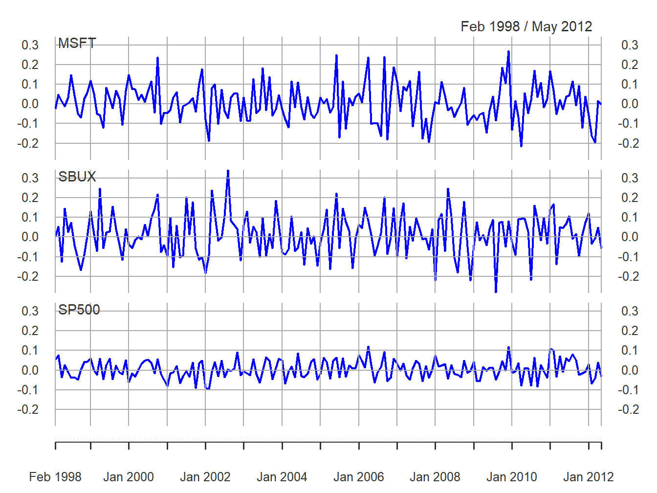
$Simulated GWN model returns on Microsoft, Starbucks and the S\&P 500 Index.$

Figure 6.11: Simulated GWN model returns on Microsoft, Starbucks and the S&P 500 Index.

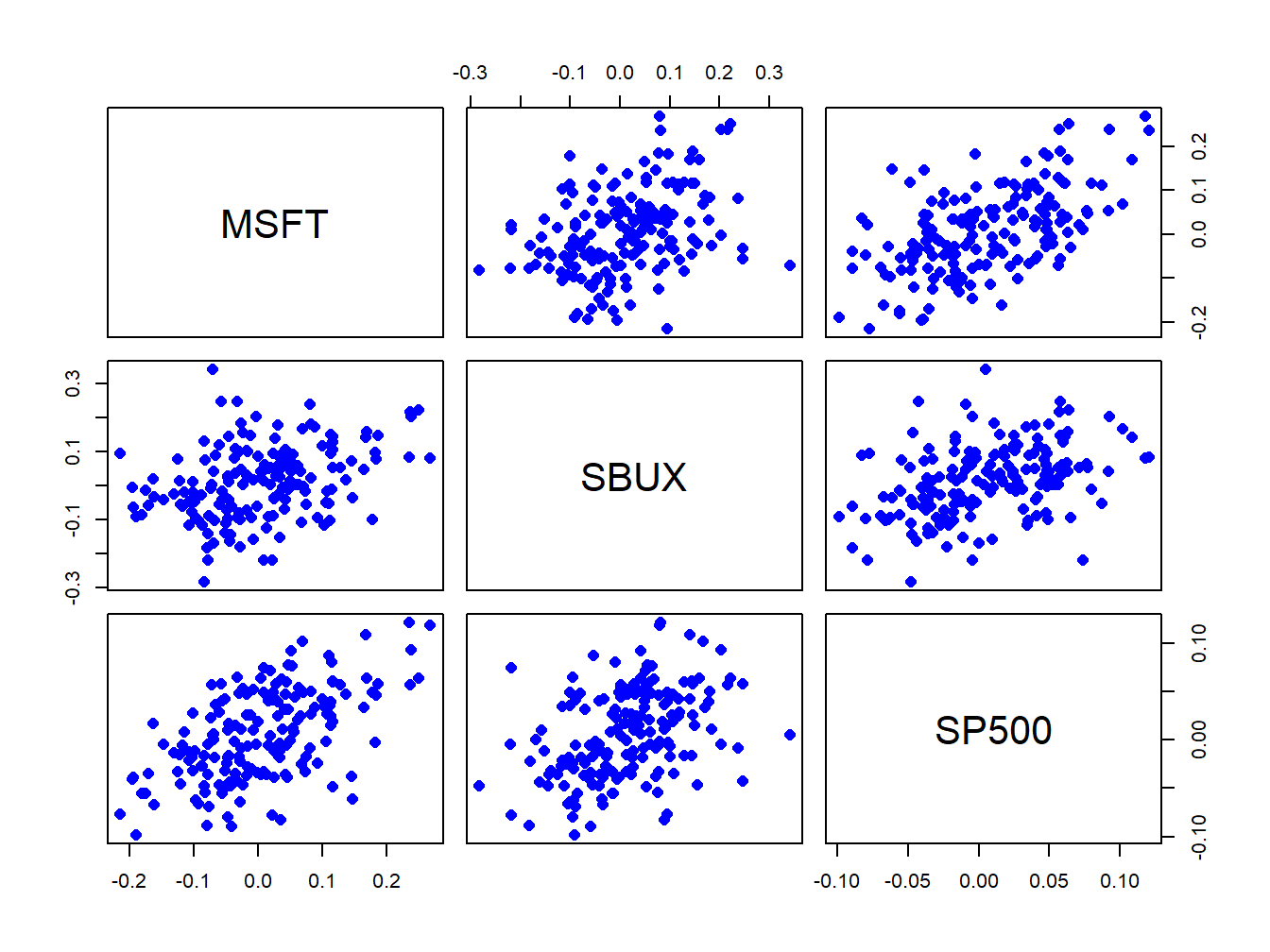
Figure 6.12: Pairwise scatterplot of simulated returns

Example 4.5 (Multiple Monte Carlo simulations of GWN model for three assets)

TBD

$\blacksquare$

Monte Carlo refers to the famous city in Monaco where gambling is legal.↩︎
Alternatively, the returns can be simulated directly by simulating observations from a normal distribution with mean $0.0$ and standard deviation 0.10.↩︎
rmvnorm returns a matrix of dimension n.obs by 3. The simulated news shocks for each asset are in the columns of e.sim. Transposing e.sim allows the mean vector to be added row-wise. Transposing again creates a column vector of simulated returns.↩︎