7.4 Estimators for the Parameters of the GWN Model
Let \(\{\mathbf{r}_{t}\}_{t=1}^{T}\) denote a sample of size \(T\) of observed returns on \(N\) assets from the GWN model (7.1). To estimate the unknown GWN model parameters \(\mu_{i},\sigma_{i}^{2}\), \(\sigma_{ij}\) and \(\rho_{ij}\) from \(\{\mathbf{r}_{t}\}_{t=1}^{T}\) we can use the plug-in principle from statistics:
Definition 7.5 The plug-in-principle says to estimate model parameters using corresponding sample statistics.
Proposition 7.3 For the GWN model parameters, the plug-in principle estimates are the following sample descriptive statistics discussed in Chapter 5:
\[\begin{align} \hat{\mu}_{i} & =\frac{1}{T}\sum_{t=1}^{T}r_{it},\tag{7.11}\\ \hat{\sigma}_{i}^{2} & =\frac{1}{T-1}\sum_{t=1}^{T}(r_{it}-\hat{\mu}_{i})^{2},\tag{7.12}\\ \hat{\sigma}_{i} & =\sqrt{\hat{\sigma}_{i}^{2}},\tag{7.13}\\ \hat{\sigma}_{ij} & =\frac{1}{T-1}\sum_{t=1}^{T}(r_{it}-\hat{\mu}_{i})(r_{jt}-\hat{\mu}_{j}),\tag{7.14}\\ \hat{\rho}_{ij} & =\frac{\hat{\sigma}_{ij}}{\hat{\sigma}_{i}\hat{\sigma}_{j}}.\tag{7.15} \end{align}\]
The plug-in principle is appropriate because the GWN model parameters \(\mu_{i},\sigma_{i}^{2}\), \(\sigma_{ij}\) and \(\rho_{ij}\) are characteristics of the underlying distribution of returns that are naturally estimated using sample statistics.
The plug-in principle sample statistics (7.11) - (7.15) are given for a single asset and the statistics (7.14) - (7.15) are given for one pair of assets. However, these statistics can be computed for a collection of \(N\) assets using the matrix sample statistics:
\[\begin{align} \underset{(N\times1)}{\hat{\mu}} & =\frac{1}{T}\sum_{t=1}^{T}\mathbf{r}_{t}=\left(\begin{array}{c} \hat{\mu}_{1}\\ \vdots\\ \hat{\mu}_{N} \end{array}\right),\tag{7.16}\\ \underset{(N\times N)}{\hat{\Sigma}} & =\frac{1}{T-1}\sum_{t=1}^{T}(\mathbf{r}_{t}-\hat{\mu})(\mathbf{r}_{t}-\hat{\mu})^{\prime}=\left(\begin{array}{cccc} \hat{\sigma}_{1}^{2} & \hat{\sigma}_{12} & \cdots & \hat{\sigma}_{1N}\\ \hat{\sigma}_{12} & \hat{\sigma}_{2}^{2} & \cdots & \hat{\sigma}_{2N}\\ \vdots & \vdots & \ddots & \vdots\\ \hat{\sigma}_{1N} & \hat{\sigma}_{2N} & \cdots & \hat{\sigma}_{N}^{2} \end{array}\right).\tag{7.17} \end{align}\]
Here \(\hat{\mu}\) is called the sample mean vector and \(\hat{\Sigma}\) is called the sample covariance matrix. The sample variances are the diagonal elements of \(\hat{\Sigma}\), and the sample covariances are the off diagonal elements of \(\hat{\Sigma}.\) To get the sample correlations, define the \(N\times N\) diagonal matrix: \[ \mathbf{\hat{D}}=\left(\begin{array}{cccc} \hat{\sigma}_{1} & 0 & \cdots & 0\\ 0 & \hat{\sigma}_{2} & \cdots & 0\\ \vdots & \vdots & \ddots & \vdots\\ 0 & 0 & \cdots & \hat{\sigma}_{N} \end{array}\right). \]
Then the sample correlation matrix \(\mathbf{\hat{C}}\) is computed as:
\[\begin{equation} \mathbf{\hat{C}}=\mathbf{\hat{D}}^{-1}\mathbf{\hat{\Sigma}}\mathbf{\hat{D}}^{-1} = \left(\begin{array}{cccc} 1 & \hat{\rho}_{12} & \cdots & \hat{\rho}_{1N}\\ \hat{\rho}_{12} & 1 & \cdots & \hat{\rho}_{2N}\\ \vdots & \vdots & \ddots & \vdots\\ \hat{\rho}_{1N} & \hat{\rho}_{2N} & \cdots & 1 \end{array}\right).\tag{7.18} \end{equation}\]
Here, the sample correlations are the off diagonal elements of \(\mathbf{\hat{C}}\).
To illustrate typical estimates of the GWN model parameters, we use data on monthly simple and continuously compounded (cc) returns for Microsoft, Starbucks and the S & P 500 index over the period January 1998 through May 2012 from the IntroCompFinR package. This is same data used in Chapter 5 and is constructed as follows:
data(msftDailyPrices, sp500DailyPrices, sbuxDailyPrices)
msftPrices = to.monthly(msftDailyPrices, OHLC=FALSE)
sp500Prices = to.monthly(sp500DailyPrices, OHLC=FALSE)
sbuxPrices = to.monthly(sbuxDailyPrices, OHLC=FALSE)
# set sample to match examples in other chapters
smpl = "1998-01::2012-05"
msftPrices = msftPrices[smpl]
sp500Prices = sp500Prices[smpl]
sbuxPrices = sbuxPrices[smpl]
# calculate returns
msftRetS = na.omit(Return.calculate(msftPrices, method="simple"))
sp500RetS = na.omit(Return.calculate(sp500Prices, method="simple"))
sbuxRetS = na.omit(Return.calculate(sbuxPrices, method="simple"))
msftRetC = log(1 + msftRetS)
sp500RetC = log(1 + sp500RetS)
sbuxRetC = log(1 + sbuxRetS)
# merged data set
gwnRetS = merge(msftRetS, sbuxRetS, sp500RetS)
gwnRetC = merge(msftRetC, sbuxRetC, sp500RetC)
colnames(gwnRetS) = colnames(gwnRetC) = c("MSFT", "SBUX", "SP500")
These data are illustrated in Figures 7.2 and 7.3.
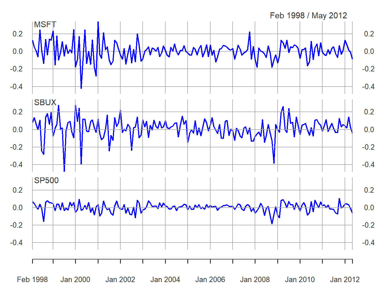
Figure 7.2: Monthly cc returns on Microsoft stock, Starbucks stock, and the S&P 500 index, over the period January 1998 through May 2012.
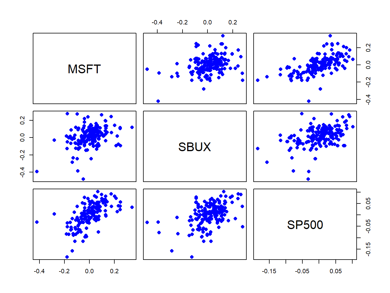
Figure 7.3: Monthly cc returns on Microsoft stock, Starbucks stock, and the S&P 500 index, over the period January 1998 through May 2012.
The estimates of \(\mu_{i}\) (\(i=\textrm{msft,sbux,sp500})\) using
(7.11) or (7.16) can be computed using
the R functions apply() and mean():
##    MSFT    SBUX   SP500
## 0.00413 0.01466 0.00169
Starbucks has the highest average monthly return at 1.5% and the S&P 500 index has the lowest at 0.2%.
The estimates of the parameters \(\sigma_{i}^{2},\sigma_{i}\), using
(7.12) and (7.13) can be computed using
apply(), var() and sd():
##           MSFT   SBUX   SP500
## sigma2hat 0.01 0.0125 0.00235
## sigmahat  0.10 0.1116 0.04847
Starbucks has the most variable monthly returns at 11%, and the S&P 500 index has the smallest at 5%.
The scatterplots of the returns are illustrated in Figure 7.3.
All returns appear to be positively related. The covariance and correlation
matrix estimates using (7.17) and (7.18) can
be computed using the functions var() (or cov())
and cor():
##          MSFT    SBUX   SP500
## MSFT  0.01004 0.00381 0.00300
## SBUX  0.00381 0.01246 0.00248
## SP500 0.00300 0.00248 0.00235## MSFT SBUX SP500
## MSFT 1.000 0.341 0.617
## SBUX 0.341 1.000 0.457
## SP500 0.617 0.457 1.000To extract the unique pairwise values of \(\sigma_{ij}\) and \(\rho_{ij}\)
from the matrix objects covmat and cormat use:
covhat = covmat[lower.tri(covmat)]
rhohat = cormat[lower.tri(cormat)]
names(covhat) <- names(rhohat) <-
c("msft,sbux","msft,sp500","sbux,sp500")
covhat
## msft,sbux msft,sp500 sbux,sp500
## 0.00381 0.00300 0.00248## msft,sbux msft,sp500 sbux,sp500
## 0.341 0.617 0.457The pairs (MSFT, SP500) and (SBUX, SP500) are the most correlated. These estimates confirm the visual results from the scatterplot matrix in Figure 7.3.
\(\blacksquare\)