9.2 Hypothesis Testing in the GWN Model

In this section, we discuss hypothesis testing in the context of the GWN model for asset returns:

$$\begin{align} R_{it} & =\mu_{i}+\varepsilon_{it},\,i=1\ldots,N;\,t=1,\ldots,T\tag{9.1}\\ \{\varepsilon_{it}\}_{t=1}^{T} & \sim\mathrm{GWN}(0,\sigma_{i}^{2}),\nonumber \\ \mathrm{cov}(\varepsilon_{it},\varepsilon_{js}) & =\left\{\begin{array}{c} \sigma_{ij}\\ 0 \end{array}\right.\begin{array}{c} t=s\\ t\neq s \end{array}.\nonumber \end{align}$$

In (9.1), $R_{it}$ is the monthly return (continuously compounded or simple) on asset $i$ in month $t$. Define $\mathbf{R}_{t}=(R_{1t},\ldots,R_{Nt})^{\prime}$. The GWN model in matrix form is:

$$\begin{align} \mathbf{R}_{t}=\mu+\varepsilon_{t},\tag{9.2}\\ \varepsilon_{t}\sim\mathrm{iid}~N(\mathbf{0},\Sigma).\nonumber \end{align}$$

We consider two types of hypothesis tests: (1) tests for model coefficients or functions of model coefficients; and (2) tests for model assumptions.⁵⁰ These tests can be specified for the GWN model for a single asset using (9.1), or they can be specified for the GWN model for all assets using (9.2).

9.2.1 Coefficient tests

Here, we assume that the GWM is the true model for our observed return data and we are interested in asking questions about the parameters of the model. The most common tests for model coefficients and functions of model coefficients for a single asset are tests for a specific value. Some typical hypotheses to be tested are:

$$\begin{align*} H_{0} & :\mu_{i}=\mu_{i}^{0}\text{ vs. }H_{1}:\mu_{i}\neq\mu_{i}^{0},\\ H_{0} & :\sigma_{i}=\sigma_{i}^{0}\text{ vs. }H_{1}:\sigma_{i}\neq\sigma_{i}^{0},\\ H_{0} & :\rho_{ij}=\rho_{ij}^{0}\text{ vs. }H_{1}:\rho_{ij}\neq\rho_{ij}^{0}, \\ H_{0} & :\mathrm{SR}_{i}=\mathrm{SR}_{i}^{0}\text{ vs. }H_{1}:\mathrm{SR}_{i}\neq\mathrm{SR}_{i}^{0}, \end{align*}$$

where $\mathrm{SR}_{i} = \frac{\mu_i - r_f}{\sigma_i}$ is the Sharpe ratio of asset $i$ and $r_f$ is the risk-free rate of interest. A hypothesis about the Sharpe ratio is a hypothesis about the ratio of two GWN model parameters. In the above hypotheses, the alternative hypotheses are two-sided. That is, under $H_{1}$ the model parameters are either larger or smaller than what is specified under $H_{0}$.

Also common are tests for specific sign. For example:

$$\begin{align*} H_{0} & :\mu_{i}=0\text{ vs. }H_{1}:\mu_{i}>0\text{ or }H_{1}:\mu_{i}<0,\\ H_{0} & :\rho_{ij}=0\text{ vs. }H_{1}:\rho_{ij}>0\text{ or }H_{1}:\rho_{ij}<0, \\ H_{0} & :\mathrm{SR}_{i}=0\text{ vs. }H_{1}:\mathrm{SR}_{i}>0\text{ or }H_{1}:\mathrm{SR}_{i}<0, \end{align*}$$

Here, the alternative hypotheses are one-sided. That is, under $H_{1}$ the model parameter is either greater than zero or less than zero.

Sometimes we are interested in testing hypotheses about the relationship between model coefficients for two or more assets. For example:

$$\begin{align*} H_{0} & :\mu_{1}=\mu_{2}\,\textrm{vs. } H_{1}:\mu_{1}\neq\mu_{2}, \\ H_{0} & :\mathrm{SR}_{1}=\mathrm{SR}_{2}\,\textrm{vs. } H_{1}:\mathrm{SR}_{1}\neq\ \mathrm{SR}_{2}. \end{align*}$$

It is often convenient to re-express these hypotheses in terms of differences of coefficients under the null and alternative hypotheses:

$$\begin{align*} H_{0} & :\mu_{1}-\mu_{2}=0 \,\textrm{vs. } H_{1}:\mu_{1}-\mu_{2} \neq 0, \\ H_{0} & :\mathrm{SR}_{1}-\mathrm{SR}_{2}=0 \,\textrm{vs. } H_{1}:\mathrm{SR}_{1}- \mathrm{SR}_{2} \neq 0. \end{align*}$$

9.2.2 Model specification tests

In the GWN model (9.1), asset returns are assumed to be normally distributed. The hypotheses to be tested for this assumption are:

$$\begin{align*} H_{0}: & R_{it}\sim N(\mu_{i},\sigma_{i}^{2})\,\textrm{vs. }H_{1}:R_{it}\sim\textrm{ not normal.} \end{align*}$$

Notice that the distribution of $R_{t}$ under $H_{1}$ is not specified (e.g., Student’s t with 5 degrees of freedom).

In addition, it is assumed that asset returns are uncorrelated over time. One can test the hypothesis that each autocorrelation (up to some maximum lag $J$) is zero:

$$\begin{align*} H_{0} & :\rho_{j}=\mathrm{cor}(r_{it},r_{i,t-j})=0\text{, }j=1,\ldots,J\,\mathrm{vs}.\\ H_{1} & :\rho_{j}=\mathrm{cor}(r_{it},r_{i,t-j})\neq0, \end{align*}$$

or one can test the joint hypothesis that all autocorrelation coefficients (up to some maximum lag $J$) are zero:

$$\begin{eqnarray*} H_{0}:\rho_{1} & = & \rho_{2}=\cdots=\rho_{J}=0\,vs.\\ H_{1}:\rho_{j} & \neq & 0\,\textrm{for some }j\leq J \end{eqnarray*}$$

Lastly, it is assumed that asset returns are covariance stationary. This assumption implies that all model parameters are constant over time. The hypotheses of interest are then:

$$\begin{align*} H_{0} & :\mu_{i},\sigma_{i}\text{ and }\rho_{ij}\text{ are constant over entire sample, vs.}\\ H_{1} & :\mu_{i}\text{ }\sigma_{i}\text{ or }\rho_{ij}\text{ changes in some sub-sample.} \end{align*}$$

The following sections describe test statistics for the above listed hypotheses.

9.2.3 Data for hypothesis testing examples

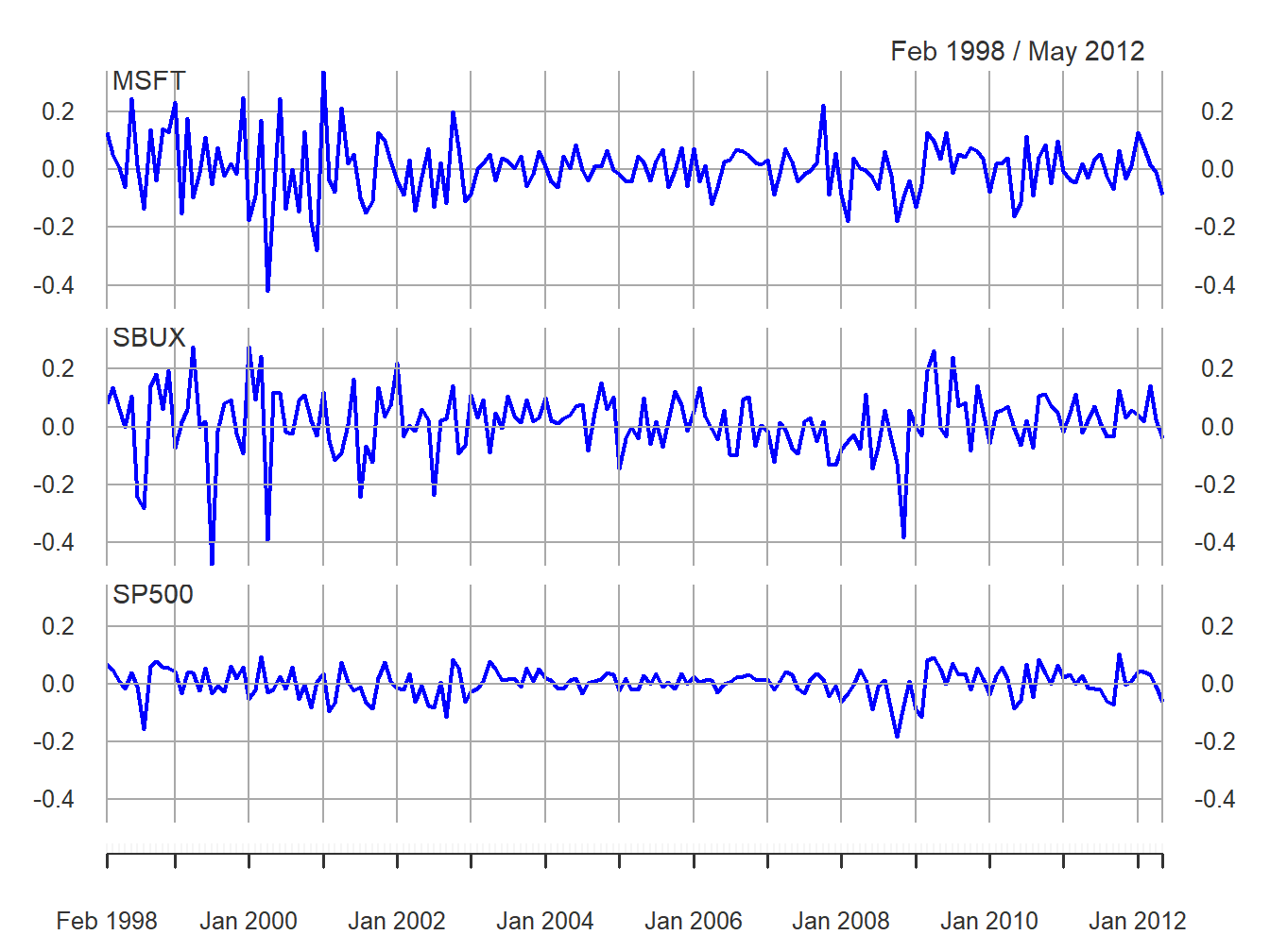
The examples in this chapter use the monthly continuously compounded returns on Microsoft, Starbucks and the S&P 500 index over the period January 1998 through May 2012 created using:

data(msftDailyPrices, sbuxDailyPrices, sp500DailyPrices) 
gwnDailyPrices = merge(msftDailyPrices, sbuxDailyPrices, sp500DailyPrices)
gwnMonthlyPrices = to.monthly(gwnDailyPrices, OHLC=FALSE) 
smpl = "1998-01::2012-05" 
gwnMonthlyPrices = gwnMonthlyPrices[smpl] 
gwnMonthlyRetC = na.omit(Return.calculate(gwnMonthlyPrices, method="log"))

The monthly continuously compounded returns, with a common y-axis, are illustrated in Figure 9.1 created using:

plot(gwnMonthlyRetC, multi.panel=TRUE, main="",
     col="blue", lwd=2, yaxis.same=TRUE,
     major.ticks="years", grid.ticks.on="years")

Figure 9.1: Monthly cc returns on Microsoft, Starbucks and the S&P 500 Index.

---

50. Tests for model assumptions are sometimes called model specification tests.↩︎